HAL Id: hal-00762845

HAL Id: hal-00762845

https://hal.archives-ouvertes.fr/hal-00762845

Submitted on 8 Dec 2012

HAL

is a multi-disciplinary open access archive for the deposit and dissemination of sci- entific research documents, whether they are pub- lished or not. The documents may come from teaching and research institutions in France or abroad, or from public or private research centers.

L’archive ouverte pluridisciplinaire

destinée au dépôt et à la diffusion de documents scientifiques de niveau recherche, publiés ou non, émanant des établissements d’enseignement et de recherche français ou étrangers, des laboratoires publics ou privés.

Tensor-based methods for numerical homogenization from high-resolution images

Loïc Giraldi, Anthony Nouy, Grégory Legrain, Patrice Cartraud

To cite this version:

Loïc Giraldi, Anthony Nouy, Grégory Legrain, Patrice Cartraud. Tensor-based methods for numerical

homogenization from high-resolution images. Computer Methods in Applied Mechanics and Engineer-

ing, Elsevier, 2013, 254, pp.154-169. �10.1016/j.cma.2012.10.012�. �hal-00762845�

Tensor-based methods for numerical homogenization from high-resolution images

L. Giraldi, A. Nouy^∗, G. Legrain, P. Cartraud

LUNAM Universit´e, GeM, UMR CNRS 6183, ´Ecole Centrale de Nantes, Universit´e de Nantes, France

Abstract

We present a complete numerical strategy based on tensor approximation techniques for the solution of numerical homogenization problems with geometrical data coming from high resolution images. We first introduce specific numerical treatments for the translation of image-based homogenization problems into a tensor framework. It includes the tensor approximations in suitable tensor formats of fields of material properties or indicator functions of multiple material phases recovered from segmented images. We then introduce some variants of Proper Generalized Decomposition (PGD) methods for the construction of tensor decompositions in different tensor formats of the solution of boundary value problems. A new definition of PGD is introduced which allows the pro- gressive construction of a Tucker decomposition of the solution. This tensor format is well adapted to the present application and improves convergence properties of tensor decompositions. Finally, we use a dual-based error estimator on quantities of interest which was recently introduced in the context of PGD. We exhibit its specificities when it is used for assessing the error on the homogenized properties of the heterogeneous material. We also provide a complete goal-oriented adaptive strategy for the progres- sive construction of tensor decompositions (of primal and dual solutions) yielding to predictions of homogenized quantities with a prescribed accuracy.

Keywords: Image-based computing, Numerical Homogenization, Tensor methods, Proper Generalized Decomposition (PGD), Model Reduction, Goal-oriented error estimation, Adaptive approximation

Introduction

With the development of affordable high resolution imaging techniques, such as X-ray microtomography, high resolution geometrical characterization of material microstruc- tures is increasingly used in industry. However, the amount of informations that are available is still difficult to handle in numerical models. This is why dedicated approaches

IThis work is supported by the French National Research Agency (grant ANR-2010-COSI-006-01).

∗Corresponding Author

Email addresses: [email protected](L. Giraldi),[email protected](A.

Nouy),[email protected](G. Legrain),[email protected](P. Cartraud) Preprint submitted to Computer Methods in Applied Mechanics and Engineering October 27, 2012

have been proposed in order to incorporate these informations for simulation purposes [57]. The most used approach in this context is the voxel-based finite element method introduced in [21,25], where each voxel of the model is transformed into a finite element.

The approach is straightforward and automatic for the generation of the computational model (see [43] for a review). However, it leads to huge numerical models, as the number of elements corresponds to the number of voxels in the image (in the order of 8 billion of elements for a full resolution 2000×2000×2000 voxels CT scan). In addition, the representation of the interfaces is not smooth, which induces local oscillations in the mechanical fields [9, 40, 53]. The size of the model can be decreased with the use of an octree coarsening away from the interfaces [40] or by decreasing the resolution of the image [3, 38, 42]. However, this can severely decrease the geometrical accuracy (more jagged interfaces) and increase the oscillations. In order to get rid of these oscillations, mesh smoothing techniques can be considered, e.g. [6]. Ultimately, full resolution images can still be considered, using Fast Fourier Transforms (FFT) algorithms [44] in the case of periodic problems.

A second class of approaches consists in extracting the material interfaces from the image and then in constructing an unstructured conforming mesh from these informa- tions, e.g. [41, 56, 57]. This allows to generate smooth interfaces and adapt the mesh in order to master the size of the model. However, meshing complex geometries is still difficult and usually requires human guidance.

Finally, non-conforming approaches can be considered (see [13, 54] among others):

these approaches allows to avoid meshing issues. In particular, the eXtended Finite Element Method (X-FEM) has been used by the authors for the treatment of 2D and 3D image-based analysis [35, 36,40]. An integrated approach was proposed in order to incorporate the geometrical informations into the numerical model. It is based on the use of Level-set functions [51], for both segmentation and mechanical analysis. Thanks to the use of tailored enrichment functions, it is possible to represent the interfaces on a non- conforming mesh. The size of the numerical model is decreased thanks to the use of an octree database that enables to keep maximum geometrical accuracy near the interfaces.

This allows to obtain a good compromise between easy mesh generation and accuracy (both geometrical and mechanical). More recently, an improvement was proposed by the use of a high-order two mesh strategy that enables high geometrical and mechanical accuracy on coarse meshes [37].

Despite of the improvements in the numerical efficiency of the methods discussed above, image-based computations are still computationaly demanding, leading to time consuming studies especially for large resolution images. There is still a need for new approaches that would allow the efficient resolution of such large scale problems.

This is why an alternative path is proposed in this paper. It relies on the use of tensor approximation methods for the solution of image-based homogenization problems. The basic idea is to interpret 2 or 3-dimensional fields as 2 or 3-order tensors, and to use ten- sor approximation methods for the approximate solution of boundary value problems.

The use of suitable tensor formats allows to drastically reduce the computational costs (time and memory storage) and therefore allows the computation on very high resolu- tion images. This paper provides a complete tensor-based numerical methodology, going from the translation of homogenization problems into a tensor framework, to the devel- opment of a goal-oriented adaptive construction of tensor decompositions based on error

2

estimation methods, and dedicated to the present application.

We first translate image-based homogenization problems to a tensor framework by in- troducing suitable tensor approximations of geometrical data. Tensor approximation methods are applied to indicator functions of material phases, which are previously smoothed in order to improve the convergence properties of their decompositions. Suit- able weak formulations of boundary value problems preserving tensor format are intro- duced in order to handle the different types of boundary conditions that are used in classical numerical homogenization methods. Regarding the construction of tensor ap- proximations of the solution of PDEs, we use Proper Generalized Decomposition methods (PGD), which is a family of methods for the construction of tensor decompositions with- out a priori information on the solution of the PDE [10,28,45, 46] (see [12] for a short review on PGD methods). Theoretical convergence properties have been recently ob- tained for a class of PGD algorithms [7, 15,16]. Note that a basic PGD algorithm has been used in [11] for the numerical solution of PDEs with heterogeneous materials whose geometry is easily represented in a tensor format. The method has also been used for deriving efficient non-concurrent non-linear homogenization strategies [31].

Although PGD methods rely on general concepts in approximation of tensors, practical algorithms have only been provided for the approximation in canonical tensor format.

However, this format is known to have bad topological properties yielding ill-posedness of best approximation problems in the set of rank-rcanonical tensors ford >2 andr >1 [52]. Greedy constructions of canonical tensor decompositions allow to circumvent this issue but present only poor convergence properties. Here, we introduce variants of PGD algorithms for the construction of tensor decompositions in different tensor formats. In particular, we introduce a new definition of PGD which allows the progressive construc- tion of a Tucker approximation of the solution. This tensor format is well adapted to the present application and yields to improved convergence properties of tensor decom- positions. The subset of Tucker tensors with bounded rank is known to possess nice topological properties yielding well posedness and numerical stability of best approxima- tion problems in these subsets [14]. Moreover, efficient algorithms based on SVD have been proposed for computing quasi-optimal Tucker approximations of a tensor, with controlled precision [34]. The algorithm proposed in this paper can be interpreted as an adaptive subspace-based model reduction method which consists in constructing a se- quence of reduced approximation spaces extracted from successive rank-one corrections.

An approximation (in Tucker format) is then obtained by a projection on the tensor product of these approximation spaces. The main drawback of the use of Tucker tensors is that it suffers from the curse of dimensionality. For dimensiond >3, a recent format coined “hierarchical Tucker tensors” [19] combines the advantages of the canonical and the Tucker tensors. This work is a first step toward the use of hierarchical Tucker tensors within the PGD.

We finally devise a goal-oriented error estimation strategy in order the assess the error on quantities of interest which are the homogenized properties. Error estimation methods have been first introduced in the context of PGD in [2, 29]. Here, we use a classical dual-based error estimator (see [1]), which has been used in [2] in the context of PGD methods. The originality of the present contribution consists in providing a complete adaptive strategy for the progressive construction of tensor decompositions yielding to predictions of homogenized quantities with a prescribed accuracy. Note that the proposed adaptive strategy could also be used in other context for goal-oriented

3

approximation of PDEs in tensor formats.

The outline is as follows: Section 1 presents the homogenization problems and their variational formulations. Section2 introduces the tensor framework and notations used for separated representations. Then section3presents how the solution of PDEs can be approximated under separated representations with the PGD. In particular, we detail a new algorithm for the progressive construction of a Tucker decomposition. Next, image geometry and boundary conditions are expressed in a tensor format in section4. First numerical examples are introduced in section5. Then, in section6, we introduce a goal- oriented adaptive algorithm using error estimators on homogenized properties. Finally, the article presents an application on a cast iron image extracted from a tomography, where we use the complete goal-oriented adaptive solution method.

1. Homogenization problems and variational formulations

In this section, we introduce classical homogenization methods for a linear heat diffu- sion problem. Homogenization problems are boundary value problems formulated on a domain Ω which constitutes a representative volume of an heterogeneous material. The solution of these problems allows to extract effective for apparent macroscopic properties of the material depending on whether Ω is larger than the representative volume element (RVE). Note however that the prediction of the size of the representative volume is out of the scope of this paper. The reader can refer to [23, 24,39, 48] for methodologies to estimate the size of the representative volume. In the following, we will identify both apparent and homogenized properties.

1.1. Scale transition and localization problems

We denote by uand qthe temperature and flux fields respectively. The macroscopic gradient of the field ∇u^M and the macroscopic flux q^M are defined through a spatial averaging of the corresponding microscopic quantities∇uand qover the representative volume Ω:

∇u^M =<∇u >= 1

|Ω|

Z

Ω

∇u dΩ (1)

q^M =< q >= 1

|Ω|

Z

Ω

q dΩ (2)

The inverse process yielding the microscopic fields from the macroscopic ones is called localization. Given ∇u^M or q^M, microscopic fields ∇u and q are obtained by solving localization problems which are boundary value problems defined on Ω:







∇ ·q(x) = 0 on Ω

q(x) =−K(x)· ∇u(x) on Ω

+ boundary conditions depending on∇u^M orq^M

(3)

whereK is the conductivity field. If the data is the macroscopic gradient ∇u^M or the macroscopic fluxq^M, we obtain the microscopic fields respectively by

∇u(x) =A(x)· ∇u^M (4)

4

or

q(x) =B(x)·q^M (5)

whereA and B are called localization tensors. Once we have obtained the microscopic fields through equations (4) (resp. (5)) for a given∇u^M (resp. q^M), we can deduce the other macroscopic fieldq^M (resp. ∇u^M) by using the constitutive relation and a spatial averaging. We finally define the effective (homogenized) conductivity tensor K_h such that

q^M =−K

h· ∇u^M (6)

1.2. Boundary conditions

The homogenized conductivity tensor depends on the localization process which is governed by the choice of the boundary conditions. These boundary conditions are expressed as a function of a macroscopic field which is the input data of the microscopic problem. Classically, three sets of boundary conditions are considered [22–24,49]. They are described below.

1.2.1. Natural Boundary Conditions (NBC)

Boundary value problem (3) is considered with the following Neumann boundary con- ditions:

q(x)·n=q^M·n on∂Ω (7)

withq^M given andnthe outer pointing normal of∂Ω. The solutionuis a priori defined up to a constant. A well-posed problem can be obtained by introducing the following solution space

H_m¹(Ω) =

v∈H¹(Ω);

Z

Ω

v dΩ = 0

(8) The weak formulation of the problem is then:

Findu∈H_m¹(Ω) such that

∀δu∈H_m¹(Ω), Z

Ω

∇δu·K· ∇u dΩ =− Z

∂Ω

δu q^M·n dΓ (9) Using equation (5), we obtain

∇u^M =<∇u >=<−K⁻¹·q >=−< K⁻¹·B >· q^M :=−(K^nbc

h )⁻¹·q^M (10) Then, the solutions obtained from 3 different values ofq^M (e.g. (1,0,0)^T, (0,1,0)^T and (0,0,1)^T) yield the complete characterization ofK^nbc

h . 1.2.2. Periodic Boundary Conditions (PBC)

In this case, problem (3) is considered with the following periodic boundary conditions:

u(x)− ∇u^M ·xis Ω-periodic

and q(x)·nis Ω-antiperiodic (11)

5

with∇u^M given. We denote by ˜u(x) =u(x)− ∇u^M·x. The solution ˜uis a priori defined up to a constant. A well-posed problem can be obtained by introducing the following solution space

H_per,m¹ (Ω) =

v∈H_per¹ (Ω);

Z

Ω

v dΩ = 0

(12) whereH_per¹ (Ω) is the subspace of periodic functions inH¹(Ω). The weak formulation of the problem is then:

Find ˜u∈H_per,m¹ (Ω) such that

∀δu∈H_per,m¹ (Ω), Z

Ω

∇δu·K· ∇˜u dΩ =− Z

Ω

∇δu·K· ∇u^M dΩ (13) Thanks to the linearity of the problem, ˜ucan be written as ˜u=χ· ∇u^M which yields

∇u=∇u^M+(∇χ)^T · ∇u^M = (I+ (∇ χ)^T)· ∇u^M. Thus, the localization tensor defined in equation (4) is found to be A=I+ (∇χ)^T. We thus obtain

q^M =< q >=<−K· ∇u >=−< K·(I+∇(χ)^T)>·∇u^M :=−K^pbc_h · ∇u^M (14) 3 different problems have to be solved for obtainingK^pbc_h (e.g. with∇u^M = (1,0,0)^T, (0,1,0)^T and (0,0,1)^T). It can be noticed that for a material with a periodic microstruc- ture, the localization problem defined by (3) and boundary conditions (11) can be rig- orously justified by the asymptotic expansion method [5, 33, 50]. However, note that periodic boundary conditions can be used even if the microstructure is not periodic (see e.g. [23,24]).

1.2.3. Essential Boundary Conditions (EBC)

In this case, problem (3) is considered with the following Dirichlet boundary conditions:

u(x) =∇u^M ·x on∂Ω (15)

with∇u^M given. Note that the solutionucan be expressed under the form

u(x) =∇u^M ·x+ ˜u(x) (16)

where ˜uis the solution of the following weak formulation:

Find ˜u∈H₀¹(Ω) such that

∀δu∈H₀¹(Ω), Z

Ω

∇δu·K· ∇˜u dΩ =− Z

Ω

∇δu·K· ∇u^M dΩ (17) By linearity of the problem, 3 different choices for∇u^M (e.g. (1,0,0)^T, (0,1,0)^T and (0,0,1)^T) are required to completely characterize the localization tensor A defined in equation (4). The homogenized tensorK^ebc

h is then obtained by 6.2e−3q^M =< q >=<−K· ∇u >=−< K·A >·∇u^M :=−K^ebc

h · ∇u^M (18) 6

1.3. Unified formulation

Weak formulations (9), (13) and (17) can be unified with an abuse of notation for EBC and PBC, for which ˜uis replaced byu:

Findu∈ V such that

∀δu∈ V, a(δu, u) =l(δu) (19)

with

a(δu, u) = Z

Ω

∇δu·K· ∇u dΩ

and











l(δu) =− Z

∂Ω

δu q^M ·n dΓ forNBC l(δu) =−

Z

Ω

∇δu·K· ∇u^M dΩ forPBC andEBC

(20)

Function spaceV is defined by:







V =H_m¹(Ω) forNBC V =H_per,m¹ (Ω) forPBC V =H₀¹(Ω) forEBC

(21)

The generic weak formulation (19) will be used in order to simplify the presentation of the proposed solution strategy. We will then come back to the underlying problems for detailing some technical issues and for discussing some specificities of the localization problems.

2. Tensor spaces and separated representations

In this section, we consider a scalar field of interestw: Ω→Rwhich can be the gray intensity level of the image representing the heterogeneous material, a component of the conductivity fieldK or the solution of localization problem (19). The domain Ω⊂R^d being an image, it has a product structure. We have Ω = Ω^x×Ω^y×Ω^z ford= 3 (resp.

Ω = Ω^x×Ω^yford= 2), with Ω^α= (0, l^α). In this section, and without loss of generality, we only consider the 3-dimensional case but the different notions extend naturally to arbitrary dimensiond. Under some regularity assumptions, a functionwdefined on such a cartesian domain can be identified with an element of a suitable tensor space. In this section, we introduce some general notions about tensors (as elements of tensor product spaces) and their approximation using separated representations of the form:

w(x, y, z)≈wm(x, y, z) =

m

X

i=1

v_i^x(x)v^y_i(y)v_i^z(z) (22) 7

2.1. Tensor spaces

For a general introduction to tensor spaces and tensor approximations, the reader can refer to Hackbusch [18]. We suppose thatw∈ VwhereV is a Hilbert tensor space defined in the set of functionsR^Ω. The inner product ofV is denoted<·,·>and its associated normk · k. WithV^x(resp. V^y,V^z) a Hilbert space of functions ofR^Ω

x (resp. R^Ω

y,R^Ω

z), the tensor product⊗between functions is defined in a usual way, such that

(v^x⊗v^y⊗v^z)(x, y, z) =v^x(x)v^y(y)v^z(z) (23) for allv^α∈ V^α,α∈ {x, y, z}. We define the set of rank-1 (or elementary) tensors

R₁={v=v^x⊗v^y⊗v^z;v^α∈ V^α, α∈ {x, y, z}}, (24) The algebraic tensor product⊗_a of spacesV^x,V^y andV^z is then defined by

V^x⊗aV^y⊗aV^z= span(R1) (25) Finally, the Hilbert tensor space is defined by

V=V^x⊗ V^y⊗ V^z=V^x⊗aV^y⊗aV^zk·k (26) where (·)^k·kdenotes the completion with respect to the normk · k.

In the case of a cartesian domain Ω = Ω^x×Ω^y×Ω^z, tensor spacesV that are involved in the formulation of localization problems (19), and given in (21), have the following tensor product structure:

V=V^x⊗aV^y⊗aV^{zk·kH1 (Ω)} (27)

with







V=H_m¹(Ω), V^α=H_m¹(Ω^α) forNBC V=H_per,m¹ (Ω), V^α=H_per,m¹ (Ω^α) forPBC V=H₀¹(Ω), V^α=H₀¹(Ω^α) forEBC

(28)

This justifies the existence of a separated representation of type (22) for the solution of homogenization problems (19).

2.2. Tensor decompositions

We introduce here two classical tensor decomposition formats.

Rank-m(canonical) decomposition. For a givenm∈N, the set of rank-mtensorsRmis defined by

Rm= (

wm=

m

X

i=1

vi;vi∈ R1

)

(29) Definition (26) implies that for all w∈ V, there exists a sequence of tensors, (wm)_m∈N, such thatwm∈ Rm andwm converges to w. Therefore, for anyw ∈ V, this condition justifies the existence of the approximation of type (22) with an arbitrary accuracy.

8

Tucker tensors. For a given multi-index r = (r^x, r^y, r^z) ∈ N³, we define the Tucker tensors setTras follows:

T_r=





 w_r=

r^x

X

i=1 r^y

X

j=1 r^z

X

k=1

λ_ijk v^x_i ⊗v_j^y⊗v_k^z;λ_ijk∈R, v_p^α∈ V^α, < v_p^α, v_q^α>_α=δ_pq





 (30) with < ·,· >_α the inner product on Hilbert space V^α. An approximation w_r ∈ T_r of an elementw∈ V is called a rank-rTucker approximation of w. We have the property thatRr⊂ T_(r,r,r). Therefore, for allw∈ V, there also exists a sequence (wm)_m∈N, with wm ∈ Tr_m and such that wm converges to w. The reader can refer to [27] for a review of definitions and constructions of tensor representations in finite dimensional algebraic tensor spacesV =R^Nx⊗R^Ny⊗R^Nz.

3. Proper Generalized Decomposition

The homogenization problem we want to solve has been recasted as follows (see section 1.3):

Findu∈ V such that

∀δu∈ V, a(δu, u) =l(δu) (31)

whereVis a tensor Hilbert space with tensor structure given in (28). Proper Generalized Decomposition (PGD) methods constitute a family of algorithms for the construction of a tensor approximation of the solution u of (31), without a priori information on the solution. It can be achieved by formulating best approximation problems on tensors subsets using operator-based norms instead of natural norms in tensor spaceV. In this section, we first recall the principle of PGD methods. We then introduce a now classical algorithm for the construction of rank-mapproximations and we recall some properties of this approximation. Then, we will introduce a new algorithm for the progressive construction of a Tucker representation of the solution. This algorithm provides better convergence properties than classical PGD definitions based on canonical decompositions.

Remark 1. In this section, we consider that the problems are formulated on a d- dimensional domain Ω ⊂ R^d, with Ω = Ω^x×Ω^y ×Ω^z for d = 3 or Ω = Ω^x×Ω^y ford= 2. The notation⊗α will stand for⊗_α∈{x,y,z} ford= 3 and⊗_α∈{x,y} ford= 2.

3.1. A priori definition of an approximation on a tensor subset

Let us consider a tensor subsetS (e.g. rank-1 tensors set, Tucker tensors set...). Given a normk · kinV, a best approximationu^∗∈ S ofu∈ V can be naturally defined as

ku−u^∗k= min

v∈Sku−vk (32)

The idea is to find an approximationu^∗ofuwithout a priori information onu. Therefore, the norm must be chosen in such a way that problem (32) can be solved without knowing u. In the present application, where uis solution of (31) with a a symmetric coercive and continuous bilinear form, the normk · kand associated inner product<·,·>can be chosen as follows:

kvk²=a(v, v), < u, v >=a(u, v) 9

where the normk · kis equivalent to the initial norm onV. We then have ku−vk²=a(u, u) +a(v, v)−2a(u, v) =a(u, u) +a(v, v)−2l(v), and minimization problem (32) is then equivalent to

J(u^∗) = min

v∈SJ(v), J(v) = 1

2a(v, v)−l(v) (33) We note that problem (33) that defines the tensor approximation inS does not involve the solutionu. It makes the approximation u^∗ computable without a priori information onu. Of course, tensor subsetsSmust be such that minimization problems onSare well- posed. Moreover, tensor subsetsS (such as rank-1 tensors, rank-r Tucker tensors) are manifolds which are not necessarily linear spaces, so that even if problem (31) is a linear approximation problem, minimization problem (33) is no more a linear approximation problem and specific algorithms have to be devised.

Remark 2. Note that a necessary condition for optimality ofu^∗ writes

a(u^∗, δv) =l(δv) ∀δv∈Tu^∗(S) (34) whereTu^∗(S)is the tangent linear space toS atu^∗.

3.2. Construction of a rank-m (canonical) decomposition

The aim is to find an optimal rank-m approximationum∈ Rmofuof the form um=

m

X

i=1

vi (35)

withv_i ∈ R1. A direct definition of an optimal approximation inRmwould be defined by the optimization problem (32). However, it is well known that form≥2 andd≥3, R_m is not a weakly closed set so that the minimization problem (32) is ill-posed for S=R_m[15]. A modified direct definition of an approximation with arbitrary precision ε >0 could be formulated as follows:

Findu_msuch that ku−umk ≤ inf

v∈Rm

ku−vk+ε (36)

The solution of this problem yields the whole set of rank-1 elements{vi}^m_i=1 at once. In order to avoid the introduction of the tolerance ε (i.e. ε = 0), it could be possible to consider a weakly closed subset of Rm (e.g. by adding some orthogonality constraints between rank-one elements). However, these direct constructions are computationnally expensive since when increasing m, optimization problems are defined on sets with in- creasing dimensionality and computational complexity drastically increases.

In order to circumvent the above difficulties, a progressive definition of PGD is clas- sically introduced [10, 15], which consists in building the sequence (v_i)_1≤i≤m term by term (in a greedy fashion). Even if the progressive definition is sub-optimal compared to the direct PGD approach, R1 is weakly closed [15] so that successive best approxi- mation problems onR1 are well-posed. Moreover, optimization problems on R1 have

10

Algorithm 1Progressive construction of a rank-mapproximation

1: Setu₀= 0

2: fori= 1 tomdo

3: Computew_i=⊗_αw^α_i ∈arg min

w∈R1

ku−u_i−1−wk

4: SetUi= span{wk}ⁱ_k=1

5: Computeui= arg min

v∈Ui

ku−vk

6: end for

almost the same complexity, so that the complexity of computing a rank-mapproxima- tion scales (approximately) linearly with the rankm. The algorithm used is defined in Algorithm1. Step 5 of Algorithm 1 corresponds to a classical projection onto the sub- space spanned by all rank-one elements previously generated. At step m, the solution um= arg min

v∈Um

ku−vkcan be written under the form

u_m=

m

X

i=1

λ_iw_i withw_i=⊗_αw_i^α

where the (λi)^m_i=1 ∈R^mare coefficients that are solutions of the following system of m equations:

m

X

j=1

A_ijλ_j=b_i, ∀i∈ {1, . . . , m} (37)

with

Aij =a(wi, wj) =a(⊗αv_i^α,⊗αv_j^α), bi=l(wi) =l(⊗αv_i^α)

Different algorithms have been proposed for computingwm∈arg min_v∈R1ku−u_m−1− vk (step 3). One possibility is an alternating minimization algorithm presented in Al- gorithm 2. The integer kmax represents the maximum number of iterations and the toleranceεsis associated to a stagnation criterium. In practice, we will takekmax= 10 andεs= 5.10⁻².

Remark 3. In the case wherek·kis the classical canonical norm on a finite dimensional space, Algorithm2corresponds to the Alternating Least Squares (ALS) algorithm on R1

[8,20,27].

Remark 4. If the domainΩ is 2-dimensional, the method can be considered as a gen- eralization of the SVD with respect to general norms on Hilbert spaces [15].

Minimization problem of step 5 of Algorithm 2, corresponding to the computation of v^α, is equivalent to

vmin^α∈V^α

1

2a(⊗βv^β,⊗βv^β) +a(um−1,⊗βv^β)−l(⊗βv^β) (38) 11

Algorithm 2Alternating minimization algorithm for computing wm ∈ arg min

w∈R1

ku− u_m−1−wk

1: Initialize randomlyv^α∈ V^αfor allα

2: Setw₀= 0

3: fork= 1 tok_maxdo

4: forα=x, . . .do

5: Computev^α∈arg min

v^α∈V^αku−u_m−1− ⊗_βv^βk

6: end for

7: Setwk =⊗αv^α

8: if kwk−w_k−1k/kw_k−1k< εsthen

9: break

10: end if

11: end for

12: Setwm=wk

It reduces to the solution of the following linear problem:

Findv^α∈ V^αsuch that

∀δϕ∈ V^α, a^α(δϕ, v^α) =l^α_m(δϕ) (39) with

a^α(δϕ, ϕ) =a(δϕ⊗(⊗β6=αv^β), ϕ⊗(⊗β6=αv^β)),

l_m^α(δϕ) =l(δϕ⊗(⊗β6=αv^β))−a(δϕ⊗(⊗β6=αv^β), u_m−1)

Problem (39) is a one-dimensional problem defined on V^α ⊂ H¹(Ω^α). The proposed algorithm then only involves the solution of uncoupled one-dimensional problems, which is the reason for the efficiency of the PGD method.

Remark 5. Assuming thatV^α=Rⁿ, ∀α, and that the complexity of a linear solver on a problem of sizenisn³, then the construction of all the vectors of a rank-rdecomposition with algorithm 2requires at most r kmaxd n³ operations. The update of the λ’s requires 1 + 2³+. . .+r³= ¹₄r²(r+ 1)² operations. Finally the complexity of the algorithm1 is

1

4r²(r+ 1)²+r kmaxd n³.

3.3. Construction of a rank-rTucker decomposition

An approximation of the solution using a Tucker format could be searched by solving an optimization problem:

ku−u_rk= min

v∈T_rku−vk (40)

This problem is well-posed [14]. However, this direct construction of a Tucker approx- imation ur ∈ Tr is computationally expensive and when the objective is to find an approximation with a desired accuracy, we will rather prefer an adaptive construction.

We now propose a sub-optimal but progressive construction of a sequence of Tucker approximations {um}_m∈N of the solution, where um is the best approximation of the

12

solution in a linear subspaceUmofT_(m,...,m), withUmof the form:

Um=⊗αU_m^α (41)

that meansU_m=U_m^x⊗U_m^y ⊗U_m^z for dimensiond= 3 orU_m^x ⊗U_m^y for dimensiond= 2.

Linear subspacesU_m^α ⊂ V^α are defined progressively, by completing the previous spaces U_m−1^α by fonctions w_m^α extracted from a rank-one corrections w_m = ⊗_αw_m^α of u_m−1. The sequences of linear spaces{U_m^α}_m∈N (and {Um}_m∈N) are increasing withm (with respect to inclusion). Let us detail this procedure.

LetU₀^α= 0 andU₀= 0. At iterationm, knowingu_m−1∈U_m−1=⊗_αU_m−1^α , we start by computing an optimal correctionw_m∈ R₁ofu_m−1, defined by

wm=⊗αw^α_m∈argmin

w∈R1

ku−u_m−1−wk (42)

The new linear subspaceU_m^α is then defined by

U_m^α =U_m−1^α +span{w_m^α}

which has a dimensiondim(U_m^α) := r^α_m ≤m. The linear space Um is then defined by (41) and has a dimension dim(Um) :=rm=Q

αr^α_m. The next approximationum∈Um

is then defined by the following linear approximation problem:

ku−umk= min

v∈Um

ku−vk (43)

This procedure requires the solution of a succession of best approximation problems (42) on the manifold R1, which are nonlinear approximation problems with moderate complexity, and a succession of best approximation problems on linear subspaces Um, which are approximation problems with increasing complexityrm. However, these latter problems remain classical linear approximation problems. The algorithm is summed up in Algorithm3. Step 6 (best approximation inR1) can be accomplished thanks to the Algorithm 3Progressive construction of the Tucker decomposition

1: Setu0= 0

2: forα=x, . . .do

3: SetU₀^α= 0

4: end for

5: fori= 1 tomdo

6: Computewi=⊗αw^α_i ∈arg min

w∈R1

ku−u_i−1−wk

7: forα=x, . . .do

8: SetU_i^α=U_i−1^α + span(w^α_i)

9: end for

10: Computeui= arg min

v∈Ui

ku−vk

11: end for

alternating minimization algorithm (Algorithm 2). In practice, an orthonormal basis 13

{v_j^α}_1≤j≤rα

m ofU_m^α is built using the Gram-Schmidt procedure applied to the generating set{w^α_j}_1≤j≤m. The approximationum, solution of (43), can be written under the form

um= X

i∈Im

λivi, vi=⊗αv^α_iα

withIm={i∈N^d; 1≤iα≤r^α_m}. The set of coefficients (λi)_i∈Im is solution of a linear system of equations

X

j∈Im

A_ijλ_j =b_i, i∈ Im (44)

with

Aij =a(vi, vj) =a(⊗αv^α_iα,⊗αv_j^α_α), bi=l(vi) =l(⊗αv_i^α_α)

Remark 6. The orthonormalization of basis functions allows to detect if at stepm, a new function w_m^α is contained in the previous linear space U_m−1^α , in which caseU_m^α =U_m−1^α andr^α_m=r_m−1^α . This allows to ensure the uniqueness of the best approximation um in Um(regularity of system (44)). Also, it allows to automatically detect and take part of the independence (or quasi-independence) of the solution with respect to a certain variable.

Remark 7. Again, assuming that V^α = Rⁿ, ∀α, and that the complexity of a linear solver on a problem of size n is n³, then the construction of all the vectors of a rank- (r₁, . . . , r_d)decomposition requires at mostr k_maxd n³ operations, forr₁=. . .=r_d=r.

The update of the core tensorαrequires at most 1 + 2^3d+. . .+r^3d≤r^3d+1 operations.

Finally, the complexity of the algorithm3is bounded byr^3d+1+r k_maxd n³. This indicates that we should use this method in 2D or when the geometry presents particular symmetries such that one or tworαare small compared to the others, like in section5.2for instance.

4. Tensor format for image-based homogenization problems

In order to apply the PGD method to the solution of numerical homogenization prob- lems, specific reformulations and approximations have to be introduced in order to re- cast the problem in a suitable format adapted to tensor-based methods. These specific treatments concern the separated representation of the conductivity field K, yielding an approximation of operator under a tensor format, and the introduction of suitable reformulations for imposing the different types of boundary conditions.

In [30, 31], the authors already introduced a similar computational method for ho- mogenization in the EBC case and for simple geometries. In the present contribution, these works are extended to the different boundary conditions that are classically used in computational homogenization, which necessitates the introduction of suitable reformu- lations of the variational problem. Moreover, we introduce specific numerical treatments for dealing with real geometries extracted from images.

14

4.1. Separated representation of the conductivity field

Let us consider a composite material with two phases numbered 1 and 2 in which the conductivity is constant and is denotedK

1 andK

2 respectively. IfI: Ω→ {0,1} is the characteristic function of phase 1, the local conductivityK is rewritten

K(x) =I(x)K

1+ (1−I(x))K

2=K

2+I(x)

K1−K

2

Therefore, a separated representation of the scalar fieldI∈L²(Ω) =⊗αL²(Ω^α) yields a separated representation ofK. Suppose that the image containsP^x×P^y×P^z voxels ford= 3, orP^x×P^ypixels ford= 2. Ford= 3, the discrete characteristic function can be written

I(x, y, z) =

P^x

X

i=1 P^y

X

j=1 P^z

X

k=1

Iijkφ^x_i(x)φ^y_j(y)φ^z_k(z) (45) whereIijk is the value ofI in the voxel (i, j, k) and where the{φ^α_i}_1≤i≤P^α are piecewise constant interpolation functions. Ford= 2, we can write

I(x, y) =

P^x

X

i=1 P^y

X

j=1

I_ijφ^x_i(x)φ^y_j(y) (46) whereI_ij is the value ofIin the pixel (i, j). We then identify functionIwithI= (I_ijk)∈ R^P

x⊗R^P

y ⊗R^P

z ford= 3 (resp. I= (I_ij)∈R^P

x⊗R^P

y ford= 2).

In this section, we propose to slightly smooth the geometry in order to obtain a lower rank tensor decomposition. This can be seen as a particular approximation of the geom- etry. Note that voxel-based, remeshing or level-set techniques also introduce approxima- tions which result in different representations of the actual geometry.

4.1.1. Singular value decompositions We now equip ⊗_αR^P

α with the canonical inner product, which is defined for X,Y∈

⊗αR^P

α by

<X,Y>=

P^x

X

i=1 P^y

X

j=1

Xij·Yij ford= 2

<X,Y>=

P^x

X

i=1 P^y

X

j=1 P^z

X

k=1

Xijk·Yijk ford= 3

The associate norm is denotedk · k. For d= 2, it is well known that the best rank-m approximation ofIwith respect to the normk·kis the classical Singular Value Decompo- sition (SVD) truncated at rankm. Ford= 3, several alternatives have been proposed for extending the concept of SVD. One could apply the progressive PGD approach presented in section3, with the canonical normk·k, to obtain a separated representation ofI. How- ever, much more efficient constructions have been proposed for tensor decomposition in R^P

x⊗R^P

y⊗R^P

z, the tensor to be decomposed being known a priori [27]. For example, 15

the ALS algorithm computes an approximation ofIon Rm by approximating the best approximation problem onRm. We can also mention the Higher-Order Singular Value Decomposition (HOSVD) that defines an approximation of Iin the Tucker setTr. An implementation of these methods can be found in the MATLAB^TM Tensor Toolbox [4].

Note that the above definitions can be considered as particular cases of PGD methods for particular choices of norm. In fact, for the above particular norm (which is a crossnorm), these methods can be considered as multidimensional versions of the SVD.

Finally, we obtain a separated approximation Im of Iin Rm (or eventually inTrfor the Tucker format). The errorε =kI−Imk/kIk can be controlled in order to provide a desired accuracy on the description of the geometry. Note that the approximationIm

can be identified with an approximationIm ofI in the tensor spaceL²(Ω).

4.1.2. Regularized indicator functions

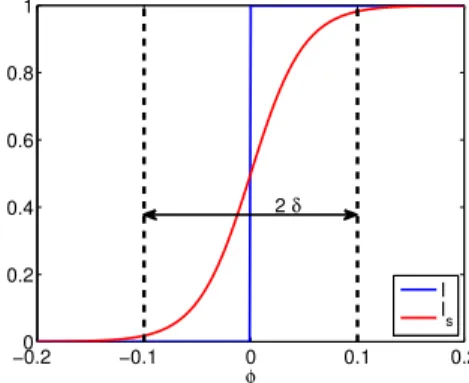
When computing a separated decomposition Im ofI using classical tensor decompo- sitions, we observe that the number of terms needed to have a good representation ofI is highly dependent on the regularity properties of functionI. The indicator function, which presents strong discontinuities at the material interfaces, is a typical example of an irregular function which yields a bad convergence of separated representations. In order to circumvent this convergence issue, the image is slightly smoothed before using tensor approximations. In practice, the iso zero of a level-setφdefined from the image is used to represent the interfaces. A smoothed indicator functionI_s is obtained by the following operation

I_s= 1 2

1 + tanh 2φ

δ

(47) whereδrepresents a characteristic length. This formula is applied on the whole level-set, no matter the distance to the interfaces. The effect of smoothing is illustrated on figure1.

−0.2 −0.1 0 0.1 0.2

0 0.2 0.4 0.6 0.8 1

φ

I I s 2 δ

Figure 1: Smoothing effect on the characteristic function

4.1.3. Illustration

We here illustrate the impact of the regularization of the indicator function on a 2D example. We consider the 2D imageI with 512×512 pixels represented in figure2. A

16

Figure 2: 2D image taken from [17]

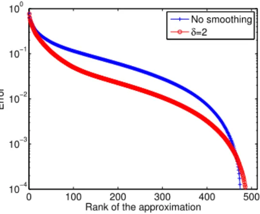
very small smoothing is applied (δ= 2 pixels). In this 2-dimensional case, the rank-m tensor approximation corresponds to a rank-mtruncated SVD. On figure 3, we illustrate the convergence of SVD applied to the original image I or to the smoothed imageIs. This figure shows that even for a small smoothing, we obtain a faster convergence of the decomposition. Indeed, for a fixed errorof 10⁻², about 100 additional modes are necessary for the decomposition of the original image. The smoothing then yields to lower

0 100 200 300 400 500

10⁻⁴ 10⁻³ 10⁻² 10⁻¹ 10⁰

Rank of the approximation

Error

No smoothing δ=2

Figure 3: Convergence inL² norm of the separated representations of the initial and smoothed images with respect to their rank.

rank representations and therefore to more efficient tensor-based algorithms. However, the smoothing introduces an approximation of the geometry that has to be controlled.

Note that another advantage of the smoothing of the characteristic function is that it removes the oscillations at the boundaries and prevents the approximation Im to be negative, which would lead to a negative conductivity in some regions of the domain and

17

therefore to an ill-posed boundary value problem.

4.2. Tensor format of boundary conditions 4.2.1. Natural Boundary conditions (NBC)

Problem (9) is reformulated as follows:

Findu∈H¹(Ω) such that∀δu∈H¹(Ω) Z

Ω

∇δu·K· ∇u dΩ +γ Z

Ω

δu dΩ Z

Ω

u dΩ =− Z

∂Ω

δu q^M ·n dΓ (48) withγ >0. For anyγ, the solution of (48) verifiesR

Ωu dΩ = 0 and therefore,u∈H_m¹(Ω) is the solution of the initial problem. We solvedproblems associated with ∇u^M =e_α, where{eα}is the canonical basis ofR^d. The right-hand side can be expressed as a sum over the boundary of the cartesian domain. The normal fluxq^M ·n being constant on each face, each term in the right-hand side is a rank-one tensor, so that the resulting right-hand side can be represented by rank-2^dtensor, where 2^dis the number of boundary faces in dimensiond.

4.2.2. Periodic Boundary Conditions (PBC) Problem (13) is first reformulated as follows:

Find ˜u∈H_per¹ (Ω) such that∀δu∈H_per¹ (Ω) Z

Ω

∇δu·K· ∇˜u dΩ +γ Z

Ω

δu dΩ Z

Ω

u dΩ =− Z

Ω

∇δu·K· ∇u^M dΩ (49) with γ > 0. For any γ, the solution of (49) verifies R

Ωu dΩ = 0 and therefore, u ∈ H_per,m¹ (Ω) is the solution of the initial problem. The term∇u^M is uniform over Ω. The tensor format of the right-hand side then follows directly from the tensor format of the conductivity field. We solved problems associated with∇u^M =e_α, where {eα} is the canonical basis ofR^d.

The Ω-periodicity of tensor approximations of type um = Pm

i=1⊗αv^α_i is naturally obtained by imposing Ω^α-periodicity for all 1-dimensional functionsv_i^α.

4.2.3. Essential Boundary conditions (EBC)

The weak formulation of the boundary value problem associated with EBC is (17).

∇u^M being uniform on Ω, the tensor format of the right-hand side follows directly from the tensor format of the conductivity field. We solvedproblems associated with∇u^M = e_α, where{e_α} is the canonical basis ofR^d.

Finally, we impose homogeneous boundary conditions for all 1-dimensional functions v^α_i ∈H₀¹(Ω^α) in tensor approximations of typeum=Pm

i=1⊗αv_i^α, thus imposing homo- geneous boundary conditions forum∈H₀¹(Ω).

5. First applications

5.1. PGD using canonical tensor format

The aim is to illustrate the behavior of the progressive PGD method and estimate the impact of PGD approximations on the quality of the quantities of interest which are the homogenized tensors.

18

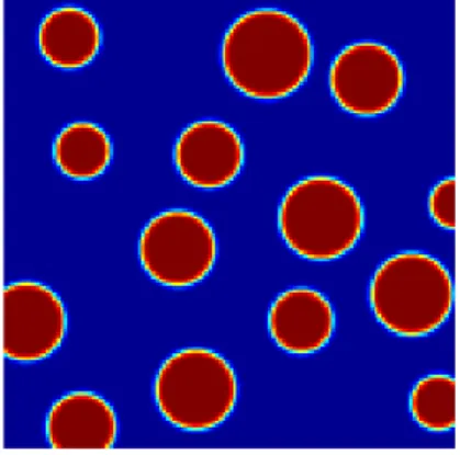
We consider the 2D image represented in figure4. The picture contains 128×128 pixels and is associated with a domain Ω = (0,1)². The domain contains random inclusions in a matrix. The materials phases are isotropic with conductivitieski= 10W.m⁻¹.K⁻¹for the inclusions andkm= 1W.m⁻¹.K⁻¹ for the matrix. We use a characteristic length of δ= 1 pixel for the smoothing of the indicator function.

Figure 4: Random inclusions into a matrix

Problem (19) has been solved for NBC, PBC and EBC using a classical Finite Element Method (FEM). These FEM solutions and the corresponding homogenized tensors are taken as reference solutions.

In order to quantify only the error coming from the PGD approximation, we use an exact representation of the original image. This avoids any degradation of the geometry due to truncation of its decomposition. We here apply a progressive PGD algorithm to construct rank-m separated representations of the solutions. On figure5 is plotted the convergence of the PGD approximations with respect to the rank of the approximation.

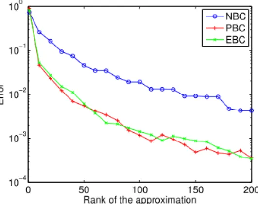
We observe similar convergence properties for different problems associated with the 3 types of boundary conditions. In fact, tensor decompositions being related to singular value decompositions (spectral decompositions), the observed convergence reflects the spectral content of the solutions. The observed plateaux can be explained by clusters of singular values. Figure6shows the convergence of the corresponding estimations of the homogenized tensors.

We can see that in the 3 cases, we have a good convergence of the homogenized tensor with the rank of the approximation. Besides, a slower convergence is observed for the NBC case. This can be explained by the fact that for the NBC case, high frequency modes in the separated approximations have non negligible spatial means, as opposed to the cases of PBC and EBC.

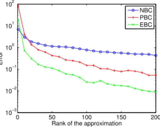
If we increase the contrast, by taking k_i= 1000W.m⁻¹.K⁻¹, we observe on figure7 a slower convergence. In figure8, we also observe a slower convergence for the homogenized tensors. The large increase of the contrast deteriorates the conditioning of the operator.

In order to improve the present results, preconditioning techniques should be introduced.

Note that some preconditioning techniques have already been introduced for operators in tensor format, see e.g. [26,32,55]. Preconditioning techniques adapted to the present framework are under investigation and will be introduced in a subsequent paper.

19

0 50 100 150 200 10⁻³

10⁻² 10⁻¹ 10⁰

Rank of the approximation

Error

Load case along x direction Load case along y direction

(a) NBC

0 50 100 150 200

10⁻³ 10⁻² 10⁻¹ 10⁰

Rank of the approximation

Error

Load case along x direction Load case along y direction

(b) PBC

0 50 100 150 200

10⁻³ 10⁻² 10⁻¹ 10⁰

Rank of the approximation

Error

Load case along x direction Load case along y direction

(c) EBC

Figure 5: Convergence of the progressive rank-mPGD approximation with respect to rankm. Relative error inL² norm.

0 50 100 150 200

10⁻⁴ 10⁻³ 10⁻² 10⁻¹ 10⁰

Rank of the approximation

Error

NBC PBC EBC

Figure 6: Relative error in canonical norm on the homogenized tensor as a function of the rank of the approximation

20

0 50 100 150 200 10⁻¹

10⁰

Rank of the approximation

Error

Load case along x direction Load case along y direction

(a) NBC

0 50 100 150 200

10⁻¹ 10⁰

Rank of the approximation

Error

Load case along x direction Load case along y direction

(b) PBC

0 50 100 150 200

10⁻¹ 10⁰

Rank of the approximation

Error

Load case along x direction Load case along y direction

(c) EBC

Figure 7: Convergence of the progressive rank-mPGD approximation with respect to rankm. Relative error inL² norm,ki= 1000W.m⁻¹.K⁻¹.

0 50 100 150 200

10⁻³ 10⁻² 10⁻¹ 10⁰ 10¹ 10²

Rank of the approximation

Error

NBC PBC EBC

Figure 8: Relative error in canonical norm on the homogenized tensor as a function of the rank of the approximation.ki= 1000W.m⁻¹.K⁻¹.

21

5.2. PGD using Tucker format

In this section we compare the convergence between the progressive PGD with canoni- cal tensor format (algorithm1) with the progressive PGD with Tucker format (algorithm 3).

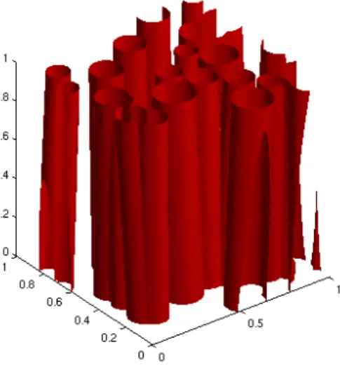
We consider the 3D image with 128³voxels represented in figure9. This image is asso- ciated with a domain Ω = (0,1)³which contains fibers in a matrix. Phases are isotropic with thermal conductivitiesk_f = 10W.m⁻¹.K⁻¹ for the fibers andk_m= 1W.m⁻¹.K⁻¹ for the matrix. The image has been separated using the Tucker ALS method from the

Figure 9: Random fibers into a matrix

MATLAB^TM Tensor Toolbox [4] with a rank-(119,119,18) Tucker decomposition, auto- matically taking into account the anisotropy of the original microstructure. The relative error inL² norm between the separated representation and the real characteristic func- tion is lower than 1%.

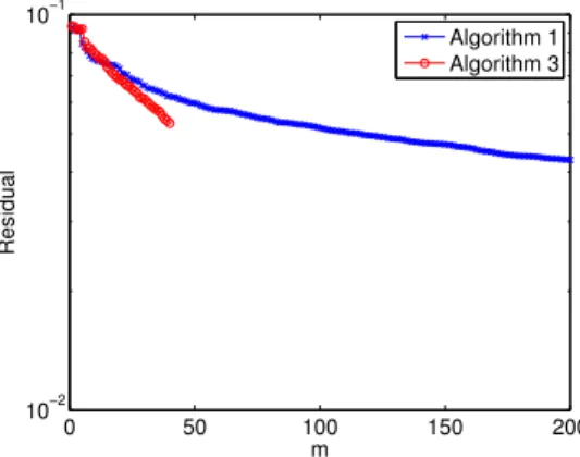
The two alternatives proposed in algorithms 1 and 3 have been tested with PBC, for the load case∇u^M = (1,0,0)^T. Here, the residual serves as an error indicator. It is plotted figure10. This figure shows that the algorithm3converges faster than1. Indeed, while 40 iterations are needed to reach a residual of 0.0532 for algorithm3, algorithm1 needs 90 iterations to reach the same value. However, algorithm3 has a much higher computational cost than algorithm1 due to the projection on the subspaces (Um)m∈N^∗. This limitation restricts the use of algorithm3to low dimensional cases (2 or 3).

Even if the residual has a poor convergence rate in both cases, we can see on figure11 that the homogenized valueK^h

xxconverges rapidly. The fast convergence of homogenized value in contrast with residual justifies the definition of new error indicators. They will be defined in the next section via goal oriented error estimation and the construction of adaptive algorithms for the solution of problem (19).

22