HAL Id: hal-01352772
https://hal.archives-ouvertes.fr/hal-01352772
Submitted on 9 Aug 2016
HAL
is a multi-disciplinary open access archive for the deposit and dissemination of sci- entific research documents, whether they are pub- lished or not. The documents may come from teaching and research institutions in France or abroad, or from public or private research centers.
L’archive ouverte pluridisciplinaire
HAL, estdestinée au dépôt et à la diffusion de documents scientifiques de niveau recherche, publiés ou non, émanant des établissements d’enseignement et de recherche français ou étrangers, des laboratoires publics ou privés.
the recovery of a potential in the wave equation.
Lucie Baudouin, Maya de Buhan, Sylvain Ervedoza
To cite this version:
Lucie Baudouin, Maya de Buhan, Sylvain Ervedoza. Convergent algorithm based on Carleman esti-
mates for the recovery of a potential in the wave equation.. SIAM Journal on Numerical Analysis,
Society for Industrial and Applied Mathematics, 2017, 55 (4), pp.1578-1613. �hal-01352772�
FOR THE RECOVERY OF A POTENTIAL IN THE WAVE
2
EQUATION.∗
3
LUCIE BAUDOUIN†, MAYA DE BUHAN‡, AND SYLVAIN ERVEDOZA§ 4
Abstract. This article develops the numerical and theoretical study of the reconstruction 5
algorithm of a potential in a wave equation from boundary measurements, using a cost functional built 6
on weighted energy terms coming from a Carleman estimate. More precisely, this inverse problem 7
for the wave equation consists in the determination of an unknown time-independent potential from 8
a single measurement of the Neumann derivative of the solution on a part of the boundary. While its 9
uniqueness and stability properties are already well known and studied, a constructive and globally 10
convergent algorithm based on Carleman estimates for the wave operator was recently proposed in 11
[BdBE13]. However, the numerical implementation of this strategy still presents several challenges, 12
that we propose to address here.
13
Key words. wave equation, inverse problem, reconstruction, Carleman estimates.
14
AMS subject classifications. 93B07, 93C20, 35R30.
15
1. Introduction and algorithms.
16
1.1. Setting and previous results. Let Ω be a smooth bounded domain of
17
Rd,d≥1 andT >0. This article focuses on the reconstruction of the potential in a
18
wave equation according to the following inverse problem:
19
Given the source termsf and f∂ and the initial data (w0, w1), con-
20
sidering the solution of
21
(1)
∂t2W −∆W+QW =f, in (0, T)×Ω,
W =f∂, on (0, T)×∂Ω,
W(0) =w0, ∂tW(0) =w1, in Ω,
22
can we determine the unknown potential Q = Q(x), assumed to
23
depend only on x∈Ω, from the additional knowledge of the flux of
24
the solution through a part Γ0 of the boundary∂Ω, namely
25
(2) M =∂nW, on (0, T)×Γ0 ?
26
Beyond the preliminary questions about the uniqueness and stability of this inverse
27
problem, already very well documented as we will detail below, we are interested in
28
the actual reconstruction of the potentialQfrom the extra information given by the
29
measurement of the fluxM of the solution on a part of the boundary. This issue was
30
already addressed theoretically in our previous work [BdBE13] based on Carleman
31
estimates. However, the algorithm proposed in [BdBE13], proved to be convergent,
32
cannot be implemented in practice as it involves minimization processes of function-
33
als containing too large exponential terms. Therefore, our goal is to address here the
34
∗Submitted to the editors DATE.
Funding:Partially supported by the Agence Nationale de la Recherche (ANR, France), Project MEDIMAX number ANR-13-MONU-0012. The authors wish to thank Institut Henri Poincar´e (Paris, France) and the Research In Paris funding.
†LAAS-CNRS, Universit´e de Toulouse, CNRS, Toulouse, France (baudouin@laas.fr)
‡CNRS, UMR 8145, MAP5, Universit Paris Descartes, Sorbonne Paris Cit, France (maya.de- buhan@parisdescartes.fr)
§Institut de Math´ematiques de Toulouse, Universit´e de Toulouse, CNRS, Toulouse, France (ervedoza@math.univ-toulouse.fr)
1
numerical challenges induced by that approach.
35 36
Before going further, let us recall that if Q ∈ L∞(Ω), f ∈ L1(0, T;L2(Ω)),
37
f∂ ∈ H1((0, T)×∂Ω), w0 ∈ H1(Ω) and w1 ∈ L2(Ω), and assuming the compati-
38
bility conditionf∂(0, x) =w0(x) for allx∈∂Ω, the Cauchy problem (1) is well-posed
39
inC0([0, T];H1(Ω))∩C1([0, T];L2(Ω)), and the normal derivative∂nW is well-defined
40
as an element ofL2((0, T)×∂Ω), see e.g. [Lio88,LLT86].
41 42
Our results will require the following geometric conditions (sometimes called “mul-
43
tiplier condition” or “Γ-condition”):
44
∃x06∈Ω, such that
45
Γ0⊃ {x∈∂Ω, (x−x0)·~n(x)≥0},
46 (3)
T >sup
x∈Ω
|x−x0|.
(4)
47
Space and time conditions (3)–(4) are natural from the observability point of view, and
48
appear naturally in the context of the multiplier techniques developed in [Ho86,Lio88].
49
They are more restrictive than the well-known observability results [BLR92] by Bar-
50
dos Lebeau Rauch based on the behavior of the rays of geometric optics, but the
51
geometric conditions (3)–(4) yield much more robust results, and this will be of pri-
52
mary importance in our approach.
53 54
In fact, under the regularity assumption
55
(5) W ∈H1(0, T;L∞(Ω)),
56
the positivity condition
57
(6) ∃α >0 such that|w0| ≥αin Ω,
58
the knowledge of ana priori boundm >0 such that
59
(7) kQkL∞(Ω)≤m, i.e. Q∈L∞≤m(Ω) ={q∈L∞(Ω),kqkL∞(Ω)≤m},
60
and the multiplier conditions (3)–(4), the results in [Baufr] (and in [Yam99] under
61
more regularity hypothesis) state the Lipschitz stability of the inverse problem con-
62
sisting in the determination of the potential Qin (1) from the measurement of the
63
fluxM in (2).
64 65
We will introduce our work by describing what was done in our former article
66
[BdBE13], in order to highlight stage by stage the main challenges when performing
67
numerical implementations.
68
In [BdBE13], we proposed a prospective algorithm to recover the potentialQfrom
69
the measurement M on (0, T)×Γ0, that we briefly recall below. We assume that
70
conditions (3)–(4) are satisfied for somex0∈/Ω, and we set β∈(0,1) such that
71
(8) βT >sup
x∈Ω
|x−x0|.
72
We then define, for (t, x)∈(−T, T)×Ω, the Carleman weight functions
73
(9) ϕ(t, x) =|x−x0|2−βt2, and forλ >0, ψ(t, x) =eλ(ϕ(t,x)+C0),
74
where C0 > 0 is chosen such that ϕ+C0 ≥ 1 in (−T, T)×Ω and λ > 0 is large
75
enough. The chore of the algorithm in [BdBE13] is the minimization of a functional
76
Ks,q[µ] given fors >0,q∈L∞≤m(Ω) andµ∈L2((0, T)×Γ0) by
77
(10) Ks,q[µ](z) = 1 2
Z T 0
Z
Ω
e2sψ|∂t2z−∆z+qz|2dxdt+s 2
Z T 0
Z
Γ0
e2sψ|∂nz−µ|2dσdt,
78
set on the trajectoriesz∈L2(0, T;H01(Ω)) such that∂2tz−∆z+qz∈L2((0, T)×Ω),
79
∂nz ∈L2((0, T)×Γ0) and z(0,·) = 0 in Ω. Note in particular that [BdBE13] shows
80
that there exists a unique minimizer of the above functional under the aforementioned
81
assumptions. The algorithm then reads as follows:
Algorithm 1(see [BdBE13])
Initialization: q0= 0 (or any guess inL∞≤m(Ω)).
Iteration: From k to k+ 1
• Step 1 -Givenqk, we setµk =∂t ∂nw[qk]−∂nW[Q]
on (0, T)×Γ0, wherew[qk] denotes the solution of (1) with the potential qk and ∂nW[Q] is the measurement given in (2).
•Step 2 -MinimizeKs,qk[µk] (defined in (10)) on the trajectoriesz∈L2(0, T;H01(Ω)) such that∂t2z−∆z+qkz∈L2((0, T)×Ω),∂nz∈L2((0, T)×Γ0) andz(0,·) = 0 in Ω.
LetZk be the unique minimizer of the functional Ks,qk[µk].
•Step 3 -Set
˜
qk+1=qk+∂tZk(0)
w0 , in Ω, wherew0 is the initial condition in (1) (recall assumption (6)).
•Step 4 -Finally, set
qk+1=Tm(˜qk+1), with Tm(q) =
q, if |q| ≤m, sign(q)m, if |q|> m, wheremis the a priori bound in (7).
82
Algorithm1comes along with the following convergence result:
83
Theorem 1 ([BdBE13, Theorem 1.5]). Under assumptions (3)-(4)-(5)-(6)-(7)-
84
(8), there exist constantsC >0,s0>0andλ >0such that for alls≥s0, Algorithm
85
1is well-defined and the iteratesqk constructed by Algorithm 1satisfy, for allk∈N,
86
(11) Z
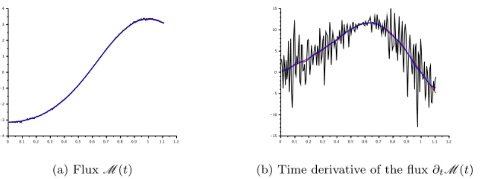
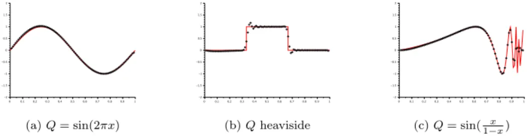
Ω
|qk+1−Q|2e2sψ(0)dx≤CkW[Q]k2H1(0,T;L∞(Ω))
s1/2α2
Z
Ω
|qk−Q|2e2sψ(0)dx.
87
In particular, for s large enough, the sequence qk strongly converges towards Q as
88
k→ ∞ inL2(Ω).
89
This algorithm presents the advantage of being convergent for any initial guessq0 ∈ L∞≤m(Ω) without any a priori guess except for the knowledge ofm. This is why we call this algorithmglobally convergent. However, while this algorithm is theoretically satisfactory as at each iteration, it simply consists in the minimization of the strictly convex and coercive quadratic functional Ks,q, it nevertheless contains several flaws and drawbacks in its numerical implementation. In particular, we underline that the functionalKs,q involves two exponentials, namely
exp(sψ) = exp(sexp(λ(ϕ+C0))),
with a choice of parameters s and λ large enough and whose sizes are difficult to estimate. In particular, for s=λ= 3 - which are not so large of course - Ω = (0,1), x0'0−,T '1+ andβ'1−, the ratio
max
(0,T)×Ω{exp(2sψ)}
min
(0,T)×Ω{exp(2sψ)}
is of the order of 10340 ! The numerical implementation of Algorithm 1 therefore
90
seems doomed.
91
The goal of this article is to improve the above algorithm so that it can fruitfully be
92
implemented. This will be achieved following several stages: working on the construc-
93
tion of the cost functional (specifically on the Carleman weight function), considering
94
the preconditioning of the cost functional, and adapting the new cost functional to
95
the discrete setting used for the numerics.
96
Before going further, let us mention that the inverse problem under consideration
97
has been well-studied in the literature, starting with the uniqueness result in the
98
celebrated article [BK81], see also [Kli92], which introduced the use of Carleman
99
estimates for these studies. Later on, stability issues were obtained for the wave
100
equation, first based on the so-called observability properties of the wave equation
101
[PY96, PY97] and then refined with the use of Carleman estimates, among which
102
[IY01a, IY01b, IY03, KY06]. In fact, a great part of the literature in this area, con-
103
cerning uniqueness, stability and reconstruction of coefficient inverse problems for
104
evolution partial differential equations can be found in the survey article [Kli13] and
105
we refer the interested reader to it. A slightly different approach can also be found in
106
the recent article [SU13] based on more geometric insights.
107
Let us also emphasize that we are interested in the case in which one performs only
108
one measurement. The question of determining coefficients from the Dirichlet to
109
Neumann map is different and we refer for instance to the boundary control method
110
proposed in [Bel97] or to methods based on the complex geometric optics, see [Isa91].
111
Here, as we said, we will focus on the reconstruction of the potential in the wave equa-
112
tion (1) from the fluxM in (2). This question has been studied only recently, though
113
the first investigation [KI95] appears in 1995, and we shall in particular point out
114
the most recent works of Beilina and Klibanov [KB12], [BK15], who study the recon-
115
struction of a coefficient in a hyperbolic equation from the use of a Carleman weight
116
function for the design of the cost functional. However, these techniques differ from
117
ours as they work on the functions obtained after a Laplace transform of the equation.
118 119
In what follows, we propose to develop a numerical algorithm in the spirit of
120
the one in [BdBE13], study its convergence and his implementation. Before going
121
further, let us also mention the fact that one can find in [CFCM13] some numerical
122
experiments based on the minimization of a quadratic functional similar to the one in
123
(10), but withsandλrather small, namelys= 1 andλ= 0.1, see [CFCM13, Section
124
4]. Our goal is to overcome this restriction on the size of the Carleman parameters,
125
as we request them to be large for the convergence of the algorithm.
126
1.2. New weight functions, new cost functionals, and a new algorithm.
127
In a first stage, we aim at removing one exponential from the cost functionalKs,q in
128
(10). Similarly to [BdBE13], looking again for a cost functional based on a Carleman
129
estimate for the wave equation, we will work with the Carleman weight function
130
exp(sϕ) instead of exp(sexp(λ(ϕ+C0))). This requires an adaptation of the proof
131
of [BdBE13] with such a weight function and the use of the Carleman estimates
132
developed in [LRS86] (see also [IY01b]), that we will briefly recall in Section2.
133
In particular, instead of minimizing Ks,q[µ] introduced in (10) as in Step 2 of
134
Algorithm 1, we will perform a minimization process on a new functional Js,q[˜µ],
135
to be defined later in (13), based on the simplified weight function exp(sϕ). Before
136
introducing that functional, we shall define the following restricted setO:
137 138
(12) O={(t, x)∈(0, T)×Ω, βt >|x−x0|}
139
={(t, x)∈(0, T)×Ω,|∂tϕ(t, x)| ≥ |∇ϕ(t, x)|},
140141
which is depicted in Figure1.
142
0 1
ϕ=0,slope
√1β
|x−x0|=βt, slop e
1 β
O
x0 x
T t
Ω
Fig. 1: Illustration of domainOin the case Ω = (0,1).
Fors >0,q∈L∞(Ω) and ˜µ∈L2((0, T)×Γ0), we then introduce the functional
143
Js,q[˜µ] defined by
144 145
(13) Js,q[˜µ](z) = 1 2
Z T 0
Z
Ω
e2sϕ|∂t2z−∆z+qz|2dxdt
146
+s 2
Z T 0
Z
Γ0
e2sϕ|∂nz−µ|˜2dσdt+s3 2
Z Z
O
e2sϕ|z|2dxdt,
147 148
to be compared with Ks,q[µ] in (10), on the trajectories z ∈ C0([0, T];H01(Ω)) ∩ C1([0, T];L2(Ω)) such that∂t2z−∆z+qz∈L2((0, T)×Ω) andz(0,·) = 0 in Ω.
This functional Js,q[˜µ] is quadratic, and as we will show later in Section 2.3, under conditions (3)–(4)–(8), it is strictly convex and coercive, therefore enjoying similar properties as the functional Ks,q[µ]. Nevertheless, let us once more emphasize that the functionalJs,q[˜µ] is less stiff than the functionalKs,q[µ] as now the weights are of the form exp(2sϕ) instead of exp(2sψ) = exp(2sexp(λ(ϕ+C0))) in (10). This already indicates the possible gain we could have by working with the functional Js,q[˜µ] in (13) instead ofKs,q[µ] in (10).
It may appear surprising to note ˜µ instead of µ. These slightly different notations come from the fact that the functionalKs,q[µ] tries to find an optimal solutionZ of
∂t2Z−∆Z+qZ '0 in (0, T)×Ω, and ∂nZ'µin (0, T)×Γ0,
while the functionalJs,q[˜µ] tries to find an optimal solution ˜Z of
∂t2Z˜−∆ ˜Z+qZ˜'0 in (0, T)×Ω, ∂nZ˜'µ˜ in (0, T)×Γ0, and Z˜'0 inO.
Therefore, as ˜Z is sought after such that it is small inO, it is natural to introduce a
149
smooth cut-off functionη∈C2(R) such that 0≤η≤1 and
150
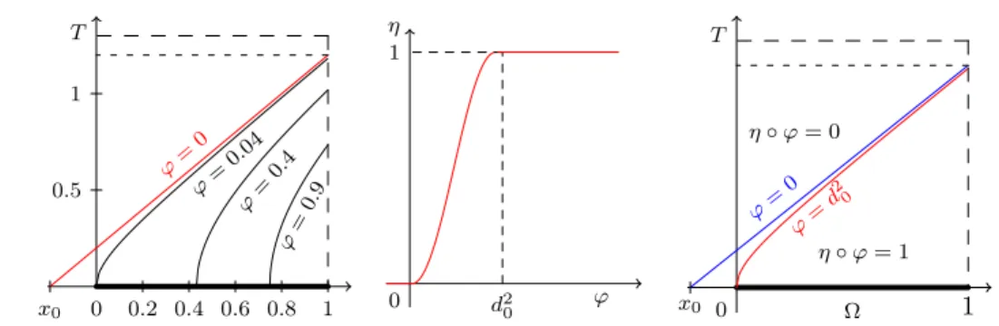
(14) η(τ) = 0, ifτ≤0, and η(τ) = 1, ifτ≥d20:=d(x0,Ω)2,
151
(recall thatd20>0 according to Assumption 3) see Figure2. Next, the idea is that if
˜
µ=η(ϕ)µ, in (0, T)×Γ0.
and ifZ denotes the minimizer of the functionalKs,q[µ] in (10), then the minimizer
152
Z˜ of Js,q[˜µ] in (13) should be close to η(ϕ)Z in (0, T)×Ω and in particular att= 0
153
this should yield, due to the choice ofη in (14),∂tZ(0)˜ '∂tZ(0) in Ω.
0.2 0.4 0.6 0.8 1 0.5
1
0
ϕ=0 ϕ=0.04
ϕ=0.4 ϕ=0.9
x0
T
0 d20 ϕ
1 η
0 ϕ=0
ϕ=d20
x0
T
η◦ϕ= 0
η◦ϕ= 1
Ω 1
Fig. 2: Isovalues of the functionϕ(x0 =−0.2,β= 1). Definition and application of the cut-off functionη.
154 155
We are then led to propose a revised version of our reconstruction algorithm,
156
detailed in Algorithm2given below.
157
Of course, if one compares Algorithm 2 with Algorithm 1, the major difference
158
is in Step 2 in which one minimizes the functional Js,qk[˜µ] in (13) instead of the
159
functional Ks,qk[µ] in (10). And as we have said above, the two functionals should
160
have minimizers that are close att= 0. In fact, similarly as Theorem1, we will obtain
161
the following result:
162
Theorem 2. Under assumptions (3)-(4)-(5)-(6)-(7)-(8), there exist positive con-
163
stants C ands0 such that for all s≥s0, Algorithm2 is well-defined and the iterates
164
qk constructed by Algorithm2 satisfy, for allk∈N,
165
(17) Z
Ω
|qk+1−Q|2e2sϕ(0)dx≤CkW[Q]k2H1(0,T;L∞(Ω))
s1/2α2
Z
Ω
|qk−Q|2e2sϕ(0)dx.
166
In particular, for s large enough, the sequence qk strongly converges towards Q as
167
k→ ∞ inL2(Ω).
168
The proof of Theorem2is given in Section2and closely follows the one of Theorem1
169
in [BdBE13]. The main difference is that the starting point of our analysis, instead
170
Algorithm 2
Initialization: q0= 0 (or any guessq0∈L∞≤m(Ω)).
Iteration: From k to k+ 1
• Step 1 - Given qk, we set ˜µk = η(ϕ)∂t ∂nw[qk]−∂nW[Q]
on (0, T)×Γ0, where w[qk] denotes the solution of
(15)
∂2tw−∆w+qkw=f, in (0, T)×Ω,
w=f∂, on (0, T)×∂Ω,
w(0) =w0, ∂tw(0) =w1, in Ω,
corresponding to (1) with the potentialqk and∂nW[Q] is the measurement in (2).
• Step 2 - We minimize the functional Js,qk[˜µk] defined in (13), for some s > 0 that will be chosen independently of k, on the trajectoriesz∈C0([−T, T];H01(Ω))∩ C1([−T, T];L2(Ω)) such that∂2tz−∆z+qkz∈L2((0, T)×Ω),∂nz∈L2((0, T)×Γ0) andz(0,·) = 0 in Ω. LetZek be the unique minimizer of the functional Js,qk[˜µk].
•Step 3 -Set
(16) q˜k+1=qk+∂tZek(0) w0
, in Ω, wherew0 is the initial condition in (15) (or (1)).
•Step 4 -Finally, set
qk+1=Tm(˜qk+1), with Tm(q) =
q, if |q| ≤m, sign(q)m, if |q| ≥m, wheremis the a priori bound in (7).
of being the Carleman estimate in [Im02], is the Carleman estimate in [LRS86].
171
The main improvement with respect to Algorithm 1 is the fact that the functional
172
Js,q[˜µ] in (13) contains weight functions with only one exponential, making the prob-
173
lem less difficult to implement. However, it is still numerically challenging to use
174
such functionals, especially as the convergence of Algorithm 2 gets better for large
175
parameters. We propose below two ideas to make it numerically tractable.
176
1.3. Preconditioning, processing and discretizing the cost functional.
177
When considering the functional Js,q[˜µ] in (13), one easily sees that exponentials
178
factors can be removed if considering the unknownzesϕinstead ofz. Such transfor-
179
mation corresponds to a preconditioning of the functional Js,q[˜µ]. Indeed, that way,
180
exponential factors do not appear anymore when computing the gradient of the cost
181
functional Js,q[˜µ]. Nevertheless, there are still exponentials factors appearing in the
182
measurements. We therefore also develop a progressive algorithm in the resolution of
183
the minimization process. The idea is to consider intervals in which the weight func-
184
tionϕdoes not significantly change, allowing to preserve numerical accuracy despite
185
the possible large values ofs. Details will be given in Section3.
186 187
When implementing the above strategy numerically, one has to discretize the
188
wave equation under consideration, and to adapt the functionalJs,q[˜µ] to the discrete
189
setting. As it is well-known [Tre82, Zua05], most of the numerical schemes exhibit
190
some pathologies at high-frequency, namely discrete rays propagating at velocity 0 or
191
blow up of observability estimates. Therefore, we need to take some care to adapt the
192
functionalJs,q[˜µ] to the discrete setting. In particular, following ideas well-developed
193
in the context of the observability of discrete waves (see [Zua05]), we will introduce a
194
naive discrete version ofJs,q[˜µ] and penalize the high-frequencies.
195
To simplify the presentation of these penalized frequency functionals, we will introduce
196
it in full details on a space semi-discrete and time continuous 1d wave equations, where
197
the space semi-discretization is done using the finite-difference method on a uniform
198
mesh. In this case, our approach, even at the discrete level, can be made completely
199
rigorous by adapting the arguments in the continuous setting and the discrete Carle-
200
man estimates obtained in [BE11] (recently extended to a multi-dimensional setting
201
in [BEO15]). We refer to Section4for extensive details.
202 203
Section 5 then presents numerical results illustrating our method on several ex-
204
amples. In particular, we will illustrate the good convergence of the algorithm when
205
the parameter sis large. We shall also discuss the cases in which the measurement
206
is blurred by some noise and the case in which the initial datum w0 is not positive
207
everywhere.
208 209
Outline. Section 2is devoted to the proof of the convergence of Algorithm2. In
210
Section3 we explain how the minimization process of the functional Js,q in (13) can
211
be strongly simplified. Section4 then makes precise the new difficulties arising when
212
discretizing the functionalJs,q, and Section5presents several numerical experiments.
213
2. Study of Algorithm 2.
214
2.1. Main ingredients. The goal of this section is to prove Theorem 2. As
215
mentioned in the introduction, the proof will closely follows the one of Theorem 1
216
in [BdBE13]. The main difference is that, instead of using the Carleman estimate
217
developed in [Im02,Baufr], we will base our proof on the following one:
218
Theorem 3. Assume the multiplier conditions (3)-(4) and β ∈(0,1) as in (8).
219
Define the weight functionϕas in(9). Then there exists0>0and a positive constant
220
M such that for all s≥s0:
221 222
(18) s Z T
−T
Z
Ω
e2sϕ |∂tz|2+|∇z|2+s2|z|2
dxdt≤M Z T
−T
Z
Ω
e2sϕ|∂2tz−∆z|2dxdt
223
+M s Z T
−T
Z
Γ0
e2sϕ|∂nz|2dσdt+M s3 Z Z
(|t|,x)∈O
e2sϕ|z|2dxdt,
224 225
for allz∈C0([−T, T];H01(Ω))∩C1([−T, T];L2(Ω))with∂t2z−∆z∈L2((−T, T)×Ω),
226
where the setO satisfies (12).
227
Furthermore, ifz(0,·) = 0inΩ, one can add to the left hand-side of (18), the following
228
term:
229
(19) s1/2
Z
Ω
e2sϕ(0)|∂tz(0)|2dx.
230
The Carleman estimate of Theorem3 is quite classical and can be found in the liter-
231
ature in several places, among which [LRS86,Isa06, Zha00, FYZ07, Bel08]. For the
232
convenience of the reader, we briefly sketch the proof in Section 2.2. However, the
233
proof of the fact that the term (19) can be added in the left hand side of (18) when
234
z(0,·) = 0 in Ω is not explicitly written in the aforementioned references, although
235
this is one of the important point of the proof of the stability result in [IY01a,IY01b].
236
Nevertheless, the idea can be adapted easily from [BdBE13], as we will detail below.
237 238
Before giving the details of the proof of Theorem2, let us first briefly explain the
239
main idea of the design of Algorithm2, which turns out to be very similar to the one
240
of Algorithm1. Indeed, both Algorithms1 and2 are constructed from the fact that
241
ifW[Q] is the solution of equation (1) andw[qk] solves (15), then
242
(20) zk=∂t w[qk]−W[Q]
243
satisfies
244
(21)
∂t2zk−∆zk+qkzk=gk, in (0, T)×Ω,
zk= 0, on (0, T)×∂Ω,
zk(0) = 0, ∂tzk(0) =z1k, in Ω,
245
wheregk = (Q−qk)∂tW[Q],z1k = (Q−qk)w0,and we haveµk=∂nzk on (0, T)×Γ0.
246
In system (21), the source gk and the initial data z1k are both unknown, and
247
we are actually interested in finding a good approximation ofz1k, which encodes the
248
information onQ−qk. In order to do so, we will try to fit “at best” the flux∂nzwith
249
µk on the boundary, approximating the unknown source termgk by 0.
250
This strategy works as we can prove that the source termgk brings less informa-
251
tion thanµkdoes, and this is where the choice of the Carleman parameterswill play
252
a crucial role. This is actually the milestone of the construction of Algorithm 1and
253
its convergence result [BdBE13]. Here, when considering the functional Js,q[η(ϕ)µ]
254
defined in (13), we rather try to approximate ˜zk =η(ϕ)zk, which enjoys the following
255
properties:
256
• ∂tz˜k(0,·) =η(ϕ(0))∂tzk(0,·) = (Q−qk)w0encodes the information onQ−qk;
257
• z˜k =η(ϕ)zk vanishes in domainO defined by (12) and on the boundary in
258
timet=T;
259
• ∂nz˜k= ˜µk in (0, T)×Γ0.
260
These ideas are actually behind the proofs of the inverse problem stability by com-
261
pactness uniqueness arguments as in [PY96,PY97,Yam99] or by Carleman estimates
262
given in [IY01a,IY01b,IY03,Baufr].
263
2.2. Sketch of the proof of the Carleman estimate. Since a lot of different
264
references, several of them mentioned right above, present detailed proof of Carleman
265
estimates for the wave equation, we only give here the main calculations yielding the
266
result presented in Theorem3.
267
Proof. Sety(t, x) =z(t, x)esϕ(t,x)for all (t, x)∈(−T, T)×Ω, and introduce the
268
conjugate operator Ls defined by Lsy =esϕ(∂t2−∆)(e−sϕy). Easy computations
269
give
270 271
(22) Lsy=∂t2y−∆y+s2(|∂tϕ|2− |∇ϕ|2)y
| {z }
=P1y
−2s∂ty∂tϕ+ 2s∇y· ∇ϕ+αsy
| {z }
=P2y 272
−s(∂t2ϕ−∆ϕ)y−αsy
| {z }
=Ry 273
274
where we have setα= 2d−2,dbeing the space dimension. Based on the estimate
275
2 Z T
−T
Z
Ω
P1yP2y dxdt≤ Z T
−T
Z
Ω
|P1y|2+|P2y|2
dxdt+ 2 Z T
−T
Z
Ω
P1yP2y dxdt
276
≤2 Z T
−T
Z
Ω
|Lsy|2dxdt+ 2 Z T
−T
Z
Ω
|Ry|2dxdt, (23)
277
the main part of the proof consists in the computation and bound from below of the cross-term
I= Z T
−T
Z
Ω
P1y P2y dxdt.
Tedious computations and integrations by parts yield
278
I=s Z T
−T
Z
Ω
|∂ty|2(∂t2ϕ+ ∆ϕ−α)dxdt+s Z T
−T
Z
Ω
|∇y|2(∂t2ϕ−∆ϕ+α+ 4)dxdt
279
+s3 Z T
−T
Z
Ω
|y|2
∂t ∂tϕ(|∂tϕ|2− |∇ϕ|2)
+α(|∂tϕ|2− |∇ϕ|2)
280
−∇ · ∇ϕ(|∂tϕ|2− |∇ϕ|2) dxdt
281
−s Z
Ω
|∂ty|2+|∇y|2
∂tϕ dx T
−T
+ 2s Z
Ω
∂ty(∇y· ∇ϕ)dx T
−T 282
−s3 Z
Ω
y2(|∂tϕ|2− |∇ϕ|2)∂tϕ dx T
−T
+αs Z
Ω
∂ty y dx T
−T 283
−s Z T
−T
Z
∂Ω
|∂ny|2∂nϕ dσdt.
284
Let us now briefly explain how each term can be estimated.
285 286
• We focus on the terms in s|∂ty|2 and s|∇y|2 in order to insure that they are
287
strictly positive. Takingα= 2d−2, this means
288
∂t2ϕ+ ∆ϕ−α=−2β+ 2d−α= 2(1−β) and
289
∂t2ϕ−∆ϕ+α+ 4 =−2β−2d+α+ 4 = 2(1−β),
290
that are positive thanks to the assumptionβ ∈(0,1).
291 292
•The terms ins3|y|2 can be rewritten as follows (since∇2ϕ= 2Id):
293
∂t ∂tϕ(|∂tϕ|2− |∇ϕ|2)
+α(|∂tϕ|2− |∇ϕ|2)− ∇ · ∇ϕ(|∂tϕ|2− |∇ϕ|2)
294
= (∂t2ϕ−∆ϕ+α)(|∂tϕ|2− |∇ϕ|2) + 2|∂tϕ|2∂t2ϕ+ 2∇2ϕ· ∇ϕ· ∇ϕ
295
= (−6β−2d+α)(|∂tϕ|2− |∇ϕ|2) + 4(1−β)|∇ϕ|2
296
=−(2 + 6β)(|∂tϕ|2− |∇ϕ|2) + 4(1−β)|∇ϕ|2.
297298
This quantity is bounded from below by a strictly positive constant in the region of (−T, T)×Ω in which
|∂tϕ(t, x)|2− |∇ϕ(t, x)|2≤0⇐⇒βt≤ |x−x0|,
i.e. the complementary of the set
(t, x)∈ (−T, T)×Ω with (|t|, x)∈ O where O
299
satisfies (12).
300 301
• We now estimate the boundary terms in time1 appearing at time t = T and
302
t =−T. We focus on the terms at timeT, as the ones at time −T can be handled
303
similarly. Let us first collect them:
304 305
IT := 2sβT Z
Ω
|∂ty(T)|2+|∇y(T)|2
dx+ 8s3βT Z
Ω
|y(T)|2(β2T2− |x−x0|2)dx
306
+ 4s Z
Ω
∂ty(T)
∇y(T)·(x−x0) +α 4y(T)
dx.
307 308
The first and second terms are obviously positive (under Condition (8) for the second
309
one), so we only need to check that they are sufficiently positive to absorb the last
310
term, whose sign is unknown. We remark that
311
Z
Ω
∇y(T)·(x−x0) +α 4y(T)
2
dx
312
= Z
Ω
|∇y(T)·(x−x0)|2 dx+α 4 Z
Ω
(x−x0)· ∇ |y(T)|2
dx+α2 16
Z
Ω
|y(T)|2dx
313
= Z
Ω
|∇y(T)·(x−x0)|2 dx+ α2
16 −αd 4
Z
Ω
|y(T)|2dx
314
≤sup
Ω
|x−x0|2 Z
Ω
|∇y(T)|2 dx,
315
sinceα= 2d−2 givesα2−4αd =−4(d−1)(d+ 1)≤0. This inequality allows to
316
deduce, by Cauchy-Schwarz inequality, that
317 318
4s Z
Ω
∂ty(T)
∇y(T)·(x−x0) +α 4y(T)
dx
319
≤2ssup
Ω
{|x−x0|}
Z
Ω
|∂ty(T)|2+|∇y(T)|2 dx
.
320 321
Using again Condition (8), we easily obtainIT ≥0.
322 323
Gathering these informations, and using the geometric condition (3) on Γ0, it
324
yields that there exists a constantM >0 independent ofssuch that
325 326
Z T
−T
Z
Ω
P1yP2y dxdt≥M s Z T
−T
Z
Ω
|∂ty|2+|∇y|2+s2|y|2 dxdt
327
−M s Z T
−T
Z
Γ0
|∂ny|2dσdt−M s3 Z Z
(|t|,x)∈O
|y|2dxdt.
328 329
1The authors acknowledge Xiaoyu Fu for having pointed out to us the fact that these boundary terms have positive signs.
From (23), we easily derive
330 331
s Z T
−T
Z
Ω
|∂ty|2+|∇y|2+s2|y|2 dxdt+
Z T
−T
Z
Ω
|P1y|2+|P2y|2 dxdt
332
≤M Z T
−T
Z
Ω
|Lsy|2dxdt+M s2 Z T
−T
Z
Ω
|y|2dxdt
333
+ M s Z T
−T
Z
Γ0
|∂ny|2dσdt+M s3 Z Z
(|t|,x)∈O
|y|2dxdt.
334 335
We take nows0large enough in order to make sure that the term ins2|y|2of the right
336
hand side is absorbed by the dominant term ins3|y|2of the left hand side as soon as
337
s≥s0 and we obtain
338 339
(24) s Z T
−T
Z
Ω
|∂ty|2+|∇y|2+s2|y|2 dxdt+
Z T
−T
Z
Ω
|P1y|2+|P2y|2 dxdt
340
≤M Z T
−T
Z
Ω
|Lsy|2dxdt+M s Z T
−T
Z
Γ0
|∂ny|2dσdt+M s3 Z Z
(|t|,x)∈O
|y|2dxdt
341 342
We then deduce (18) by substitutingy=zesϕ.
343 344
Furthermore, under the additional condition z(0,·) = 0 in Ω, we get y(0,·) = 0
345
in Ω. We then choose ρ : t 7→ ρ(t) a smooth function such that ρ(0) = 1 and ρ
346
vanishes close tot=−T. We multiply P1y byρ∂ty and integrate over (−T,0)×Ω,
347
to get
348
Z 0
−T
Z
Ω
P1y ρ∂ty dxdt= Z 0
−T
Z
Ω
∂t2y−∆y+s2((∂tϕ)2− |∇ϕ|2)y
ρ∂ty dxdt
349
= 1 2
Z 0
−T
Z
Ω
ρ∂t |∂ty|2+|∇y|2
dxdt+ s2 2
Z 0
−T
Z
Ω
ρ(|∂tϕ|2− |∇ϕ|2)∂t(y2)dxdt
350
= 1 2 Z
Ω
|∂ty(0)|2dx−1 2
Z 0
−T
Z
Ω
∂tρ |∂ty|2+|∇y|2
+s2∂t ρ(|∂tϕ|2− |∇ϕ|2) y2dxdt
351
≥ 1 2 Z
Ω
|∂ty(0)|2dx−M Z 0
−T
Z
Ω
|∂ty|2+|∇y|2+s2|y|2 dxdt.
352
By Cauchy-Schwarz inequality, this implies s1/2
Z
Ω
|∂ty(0)|2dx≤ Z T
−T
Z
Ω
|P1y|2dxdt+M s Z T
−T
Z
Ω
|∂ty|2+|∇y|2+s2|y|2 dxdt.
Using (24) andy=zesϕ, we easily deduce the estimate of term (19) and conclude the
353
proof of Theorem3.
354
From this proof of Theorem3, we can directly exhibit (see (24)) the following “con-
355
jugate” Carleman estimate, of practical interest later on:
356
Corollary 4. Assume the multiplier condition (3)-(4)andβ∈(0,1)as in (8).
357
Define the weight functionϕas in (9). Then there exist constantsM >0 ands0>0
358
such that for all s≥s0,
359 360
(25) s Z T
−T
Z
Ω
|∂ty|2+|∇y|2+s2|y|2 dxdt+
Z T
−T
Z
Ω
|P1y|2+|P2y|2 dxdt
361
≤M Z T
−T
Z
Ω
|Lsy|2dxdt+M s Z T
−T
Z
Γ0
|∂ny|2dσdt+M s3 Z Z
(|t|,x)∈O
|y|2dxdt
362 363
for all y ∈ C0([−T, T];H01(Ω))∩C1([−T, T];L2(Ω)), with Lsy ∈ L2((−T, T)×Ω),
364
whereLs,P1 andP2 are defined in (22).
365
Furthermore, ify(0,·) = 0inΩ, one can add the term s1/2 Z
Ω
|∂ty(0)|2dx to the left
366
hand-side of (25).
367
2.3. Proof of the convergence theorem.
368
Proof of Theorem 2. Let us first begin by showing that Algorithm 2 is well-
369
defined. We introduce
370 371
Tq =n
z∈C0([0, T];H01(Ω))∩C1([0, T];L2(Ω)),
372
with∂t2z−∆z+qz∈L2((0, T)×Ω) andz(0,·) = 0 in Ωo ,
373374
endowed with the norm
375 376
kzk2obs,s,q= Z T
0
Z
Ω
e2sϕ|∂t2z−∆z+qz|2dxdt+s Z T
0
Z
Γ0
e2sϕ|∂nz|2dσdt
377
+s3 Z Z
O
e2sϕ|z|2dxdt.
378 379
The proof that this quantity is a norm on Tq stems from the Carleman estimate of
380
Theorem 3 applied to ze(t, x) = z(t, x) for t ∈ [0, T] and ze(t, x) = −z(−t, x) for
381
t∈[−T,0],x∈Ω. Indeed, (18) applied tozeyields for alls≥s0,
382
s3 Z T
0
Z
Ω
e2sϕ|z|2dxdt≤2M Z T
0
Z
Ω
e2sϕ|∂t2z−∆z+qz|2dxdt
383
+ 2Mkqk2L∞(Ω)
Z T 0
Z
Ω
e2sϕ|z|2dxdt
384
+M s Z T
0
Z
Γ0
e2sϕ|∂nz|2 dσdt+M s3 Z Z
O
e2sϕ|z|2dxdt,
385
so thatk · kobs,s,qis a norm onTq providedsis large enough, and then for alls >0 as
386
the weight functions are bounded on [0, T]×Ω. This immediately implies thatJs,q[˜µ]
387
defined in (13) is coercive and strictly convex on the setTq, so that it admits a unique
388
minimizer and as a consequence, Algorithm2is well-defined.
389
Moreover, this shows that the classTq, which wasa priori dependent of q, is in
390
fact independent ofq(forq∈L∞(Ω)) and is simply given by
391 392
T =n
z∈C0([0, T];H01(Ω))∩C1([0, T];L2(Ω)),
393
with ∂t2z−∆z∈L2((0, T)×Ω) andz(0,·) = 0 in Ωo .
394395
In order to show estimate (17), instead of considering only functionals of the
396
formJs,q[˜µ], we introduce slightly more general functionalsJs,q[˜µ, g] given fors >0,
397
q∈L∞(Ω), ˜µ∈L2((0, T)×Γ0),g∈L2((0, T)×Ω) and for allz∈ T, by:
398 399
(26) Js,q[˜µ, g](z) =1 2
Z T 0
Z
Ω
e2sϕ|∂t2z−∆z+qz−g|2dxdt
400
+s 2
Z T 0
Z
Γ0
e2sϕ|∂nz−µ|˜2dσdt+s3 2
Z Z
O
e2sϕ|z|2dxdt.
401 402
With the same argument as above, the functional Js,q[˜µ, g] is coercive in the norm
403
k·kobs,s,q and strictly convex, so that it admits a unique minimizer for each ˜µ ∈
404
L2((0, T)×Γ0) andg∈L2((0, T)×Ω).
405
We then observe that ˜zk :=η(ϕ)zk, wherezk satisfies (20) (recall the definitions
406
ofη in (14) andϕin (9), pictured in Figure2), is the minimizer ofJs,qk[˜µk,˜gk] with
407
(27) ˜gk =η(ϕ)(Q−qk)∂tW[Q] + [∂t2−∆, η(ϕ)]zk,
408
since it solves:
409
(28)
∂t2z˜k−∆˜zk+qkz˜k= ˜gk, in (0, T)×Ω,
˜
zk= 0, on (0, T)×∂Ω,
˜
zk(0) = 0, ∂t˜zk(0) =η(ϕ(0,·))zk1, in Ω,
410
and∂nz˜k= ˜µk =η(ϕ)∂t ∂nw[qk]−∂nW[Q]
on (0, T)×Γ0.
411
We shall then compareZek and ˜zk, the minimizers of the functionalsJs,qk[˜µk,0]
412
andJs,qk[˜µk,˜gk] respectively, especially at the timet= 0 corresponding to the set in
413
which the information on (Q−qk) is encoded. The result is stated as follows:
414
Proposition 5. Assume the geometric and time conditions (3)-(4)onΓ0andT,
415
that β is chosen as in (8), and letµ∈L2((0, T)×Γ0) andga, gb ∈L2((0, T)×Ω).
416
Assume also thatqbelongs to L∞≤m(Ω) form >0.
417
LetZj be the unique minimizer of the functionalJs,q[µ, gj]onT forj ∈ {a, b}. Then
418
there exist positive constantss0(m)andM =M(m)such that fors≥s0(m)we have:
419
(29) s1/2 Z
Ω
e2sϕ(0)|∂tZa(0)−∂tZb(0)|2dx≤M Z T
0
Z
Ω
e2sϕ|ga−gb|2dxdt.
420
whereϕands0(m)are chosen so that Theorem3 holds.
421
We postpone the proof of Proposition5 to the end of the section and first show how
422
it can be used for the proof of Theorem2.
423 424
Recall now that ∂tz˜k(0,·) = (Q−qk)w0. Setting ˜qk+1 as in (16), we get from
425
Proposition5 applied toZa=Zek and Zb= ˜zk that
426
(30) s1/2 Z
Ω
e2sϕ(0)|˜qk+1−Q|2|w0|2dx≤M Z T
0
Z
Ω
e2sϕ|˜gk|2dxdt.
427
The next step is to get an estimates of ˜gk defined by (27). Using the fact that
428