In this sense, the constraints must be respected in every possible realization of the parameters and the objective function evaluated in the least favorable case. In the affine decision rule approach proposed in Ben-Tal et al (2004), recourse decisions are expressed as affine functions of uncertainty. On the other hand, Arslan and Detienne (2021) proposed an exact MILP reformulation of the problem in the case of linear linkage constraints involving only binary variables.
We also point out that the class of problems that can be addressed by our solution approach is quite large since we only require mild assumptions about the nature of the optimization problem in question. In Section 3, we present a relaxation of the problem, and an effective algorithm for solving it. The objective function f is a concave function of the uncertainty and a convex function of the first- and second-stage decisions, that is, fxxx,yyy : ξξξ 7→.
Proof The existence of the hyperrectangle [lll, uuu] is trivial because it is assumed that X is bounded (assumption 2.1). As in the linear and binary cases, we then replace the counterpart of constraint (3) with (6), although in the general setting this only relaxes the problem.
Relaxation
In the next proposition, we introduce a condition under which a feasible solution for problems (P) is also feasible for problem (2SRO-P). This result directly implies Corollary 2, which states that, in the special case where the first-stage variables are all binary, problem (P) is always an exact reformulation of (2SRO-P).
Enumerative algorithm
Ifv(LBp) is greater than or equal to the incumbent's cost, the node is fathomed by bounding. In the latter case, before branching, one can try to round xxxp∗; if the resulting point is inX, a feasible solution for (2SRO-P) can be calculated. In both cases we select the variable with the maximum θjp value, i.e. we select variablexj such that,.
We associate to each node the lower bound value of the current nodev(LBp) and insert it into a list of open nodes. However, the left child still allows second-stage decisions that may end up being infeasible in the original problem. An improved second stage solution may be obtained by fixing xxx =xxx∗ in problem. 2SRO-P), in the spirit of the upper bound procedure used when solving UBp.
Proposition 3 (convergence result) If F ∈ C0, our branching algorithm finally terminates or enters an infinite sequence of nodes for which the optimal solutions of the connected lower bound problems converge to the optimal solution 2SRO-P. Denote by (lllp, uuup) the connected bounds for the variables xxx and by (xxxp∗, tttp∗, yyyp∗, VVVp∗, ξξξp∗) the optimal optimal solutions of the corresponding lower bound problems. First, we show that the sequence of optimal solutions of the lower bound problems converges to the optimal solution of the lower bound problem defined by the bounds (lll∗, uuu∗).
By introducing a finite tolerance into the algorithm, we can show that an infinite branch cannot occur at any point. More specifically, given an optimal solutionxxxp∗of the lower bound problem at a nodep, we introduce the following function. Proof The proof of the previous theorem shows that there exists a subsequence P0 ⊆P that converges to a solution (xxx∗, ttt∗, yyy∗, VVV∗, ξξξ∗).
We conclude this section by observing that at each node of the branch-and-bound algorithm, the lower bound problem can be solved with ε-tolerance in a finite number of operations.
A convexification scheme based on column-generation
Since our node selection strategy always selects a node with minimal lower bound, for each node pof the branching sequence we have v(LBp) ≤v(2SRO-P) ≤ v(LB∗). Proposition 4 (Convergence to Finite Accuracy) If the branch-and-bound algorithm enters an infinite sequence of nodes, then it must converge to a pointxxx∗at which the function has a discontinuity. Then, we have {G(xxxp∗)}p∈P0 →G(xxx∗) = v(LB∗), which allows us to understand the node according to optimality after a finite number.
As shown in Ceria and Soares (1999) and Grossmann and Ruiz (2012), one can reformulate a convex disjunctive program as a compact convex MINLP by introducing an exponential number of auxiliary variables that model the disjunctions. The resulting model can thus be solved in a finite number of states using any algorithm designed for convex optimization. The resulting problem, denoted as (LBcpk), is called theRestricted Master and is formulated as follows:. LBcpk) Following the classical column generation framework, the current approximation can be improved using a so-called pricing problem defined as follows.
Note that at each iteration k, the lower bound of the optimal value of the solution (LBp) is given by v(LBcpk)−v(PPpk). This lower bound, together with the upper bound, can allow us to prematurely terminate the solution of the problem (LBp). The convergence of nonlinear column generation was found in Garc´ıa et al (2003) and implies the convergence of the final value of our method.
In this section, we report the computational results of our solution algorithm when applied to two different optimization problems, a facility location problem and a capital budgeting problem, respectively. Both problems are important from the application point of view and are defined as non-trivial variants of problems already addressed in the literature.
Facility location problem with adjustable capacity and set-up costs
We refer to problem (32) as the two-stage robust facility location problem with adjustable capacity and transportation cost setup. This problem can be cast as (2SRO-P), where the connecting constraints between the first- and second-stage variables involve pure continuous variables and exhibit convexity in the first-stage feasible space. The reader is referred to Appendix B for the derivation of the robust counterpart to ellipsoidal uncertainty sets.
To test the proposed method, a large benchmark of random instances was generated in the spirit of Cornuejols et al (1991). First, we randomly generate the location of each sitei∈V1 and customerj∈V2 using a uniform distribution in the unit square. The expected value of the variable transport costs is instead obtained by multiplying the Euclidean distance times 10.
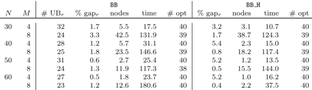
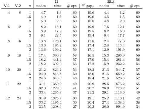
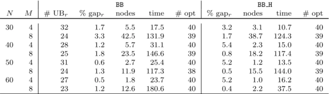
Each covariance parameter is uniformly randomly generated in the interval [σ−, σ+], where σ− and σ+ are specified below. We now report the computational results of our branch-and-bound algorithm without and with the use, at the root node, of the one-stage heuristic (SSH) of Section 3.3.3; henceforth, these versions are denoted as BB and BB H, respectively. In addition, for the BB H variant, we report in the "% gapr" column the average percent gap at the root node.
Letting LrandUr be the best lower and upper bounds at the root node, the gap is calculated as % gapr = 100 ∗ UrL−Lr. This information is omitted for algorithmBB, which never provides a feasible solution at the root node. The table shows that the complexity of these ACFL instances increases with the size of the underlying network.
Moreover, for each size of the network, increasing the value of κ (i.e. allowing for more uncertainty in the realization of the profit) makes the cases consistently harder.
Robust Capital Budgeting problem
Here, xxx are binary variables indicating whether a project has been activated in the first phase or not, while yyy indicates their activation in the second phase. Variablex0(resp.y0) is a continuous variable that indicates the fraction of the loan capacity that is activated in the first (or second) step. 2(ξξξ−gggi)TQQQi−1(ξξξ−gggi) (44) and thus expanding each conjugate appearing in the summation in (43), we get. 45) Since these terms are minimized in the objective function, any optimal solution with ti = 0 must also have sssi = 0.
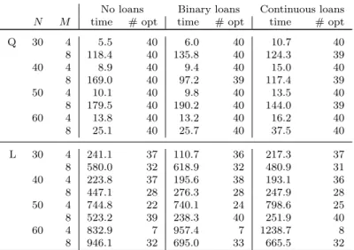
This constraint is convex as it can be modeled using a twisted square cone. Then we compute the value of the linear functiongggiTξξξat all points [−1,1]M and compute a convex quadratic function that (i) has the same value as the linear function at each node and (ii) reaches its minimum (above [−1,1]M) in one of these points. More details on this last step are in the Appendix). Each entry in the table refers to the 40 cases characterized by the same value of N and M, with the exception of those in the % gap column, which consider only cases for which a valid Uris upper limit is available.
The upper part of the table refers to cases with quadratic risk functions, while the lower part deals with the linear case. The results show that, in the quadratic case, the 'no loans' and 'binary loans' variants are generally slightly simpler than the 'continuous loans' in terms of the number of optimal solutions and the average computation time. Nevertheless, even in this challenging case, algorithmBB is able to solve almost 75% of the cases with an average time of less than 10 minutes.
In this work, we studied optimization problems where part of the cost parameters are unknown at the time of decision-making, and the decision-making process is modeled as a two-step process. For this purpose, we derive a relaxation of the problem, which can be formulated as a convex optimization problem, and embed it in a branch-and-bound algorithm, where branching occurs on integer and continuous variables. By combining counting and real-time generation of variables, we obtain a branch-price scheme for which we prove convergence to ε-optimality.
In addition to the theoretical analysis, we applied our method to two optimization problems affected by objective uncertainty, namely a variant of the Capacitated Facility Location problem and a capital budgeting problem. First, we generate linear functions (∆Li)i∈N in the same way as was done for linear cases. Furthermore, we want to ensure that the global minimum of function ∆Qi is reached at one of the extreme points of [−1,1]M.