Depending on the number of particles lost, the coils of the magnets may become normally conductive and/or be damaged. The BLM system's detectors are mainly ionization chambers located outside the cryostats.
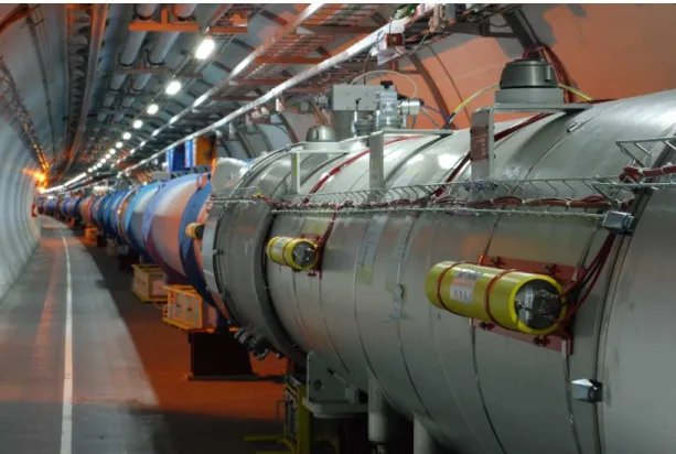
La protection du LHC
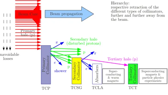
La distance entre les mors est variable, contrôlée dans la limite de 5µm et exprimée en unités de l'écart type du rayon nominal, appelé σ. Les protons déviés par les collimateurs principaux seront absorbés par d'autres collimateurs plus ouverts.
Moniteurs de perte de faisceau
Dans le rôle d'un collimateur, la position des mâchoires dans les plans transversaux (horizontal, vertical ou diagonal) joue un rôle important. Les protons absorbés créent des gerbes de particules secondaires qui seront détectées par les moniteurs de perte de faisceau.
Int´ erˆ et du travail doctoral
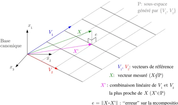
Principe de la d´ ecomposition vectorielle
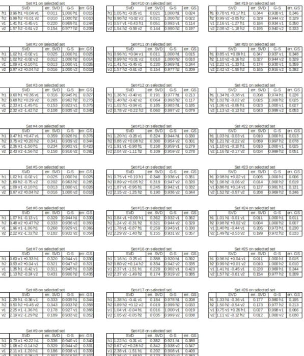
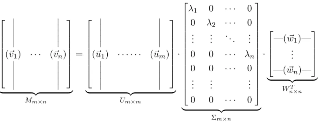
Le but de la décomposition vectorielle est de décomposer X~ en une combinaison linéaire de vecteurs (~vi), c'est-à-dire pour résoudre l'équation vectorielle : 1) Deux techniques sont utilisées pour cela : à partir d'une succession de projections vectorielles (~vi) (non orthogonales) dans l'espace vectoriel (processus de Gram-Schmidt, G-S) ; et avec des opérations matricielles. Puisque < m, la matrice des vecteurs (~vi) (notée M) n'est pas carrée et son inversion n'est pas simple.
Mise en place de la d´ ecomposition vectorielle
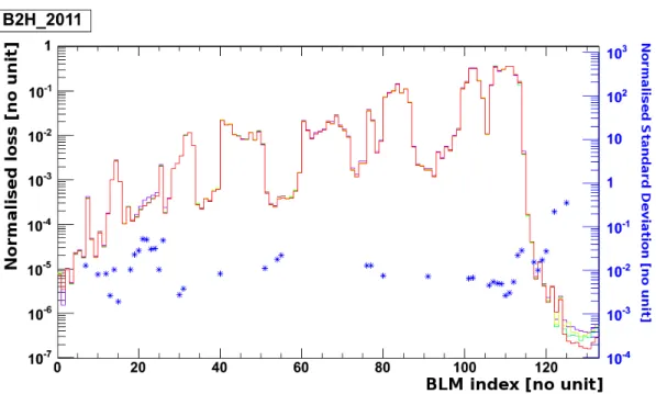
Les étoiles bleues correspondent à la valeur d’écart type normalisé pour les écrans sélectionnés. Des profils de perte pourraient être recréés en attribuant une valeur nulle aux moniteurs associés au faisceau non considéré.

Evolution temporelle
D´ ecomposition spatiale
Conclusion & Appendices
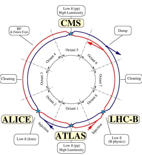
CERN
LHC PROTECTION
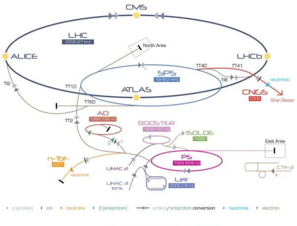
- The Large Hadron Collider
- Magnets
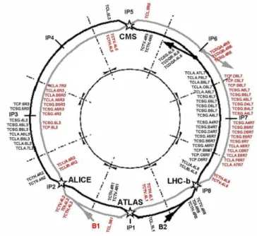
- Collimators
- Conclusion
- The monitors
They are aperture limitations: the parts of the LHC closest to the beam. The cutoff threshold values (losses above which the beam would be removed from the machine) can be tuned.
THE BLM SYSTEM
- Time Structure: Running Sums
- Electronics
- Thresholds
- Justification of the doctoral work
- Principle
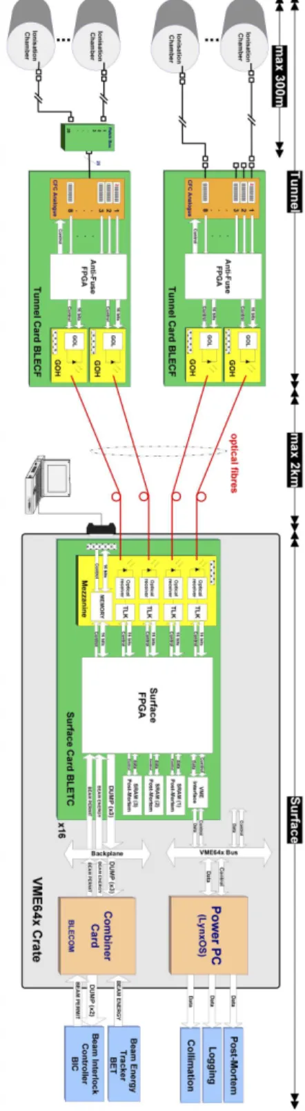
The simulation of the distribution of secondary particles according to the location of the loss is shown in fig. The input current iin(t) corresponds to the charge coming from the ionization chamber; the output is the frequency fout.
PRINCIPLE OF VECTOR DECOMPOSITION
- Singular Value Decomposition (SVD)
- Gram-Schmidt process
- MICADO
- Recomposition and error
- Conclusion
- Creation of the default vectors
However, there are not enough vectors (~vi) (n < m): they do not form a basis of the m-vector space. A negative factor in a vector decomposition indicates that the corresponding vector cannot contribute to the reconstruction of the vector X. The contribution is the projection of a vector onto another, calculated by a scalar product.
The error in the recomposition is estimated by calculating the norm of the difference between the original vector and its recomposition.
IMPLEMENTATION OF VECTOR DECOMPOSITION
Choice of the list of BLMs
In this work, each coordinate of the loss vectors corresponds to the signal of one BLM. The standard deviation quantifies the variation of the signal from one loss scenario to another. It was checked in advance whether the signal of one BLM does not change much between loss maps of the same scenario (cf. § 4.1.1).
However, both the standard deviation and the difference between minimum and maximum signals are proportional to the mean value of the signal.
Final loss map selection
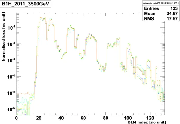
Loss cards must be sorted by another criterion: the order in which they were measured. As described in § 4.1.1, loss maps are measurements of losses during the crossing of the resonance of the melody for one of the transverse planes. The difference can already be assessed visually: there is more variation within the values of one monitor when the loss maps were measured at another location (see Figure 4.5 below).
It shows the beam 2 horizontal loss maps that were measured before the beam 2 vertical loss maps.
Adding more cases: longitudinal scenarios and TCTs
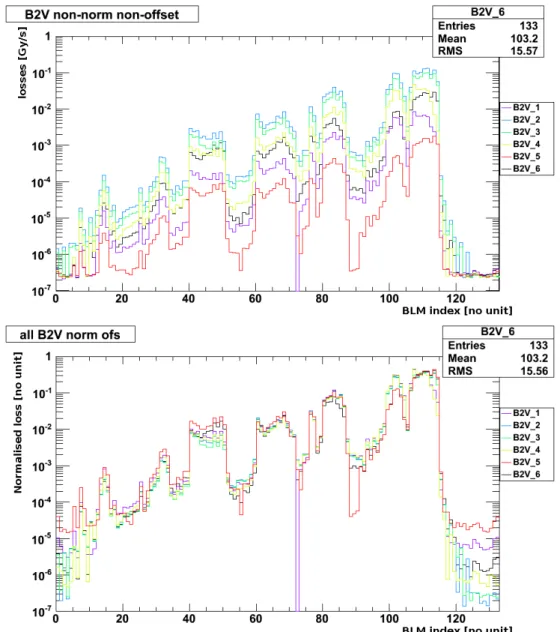
In the case of the 2011 transverse loss charts, it was shown that only the loss charts that were executed first should be kept. Most of the loss maps are mixed: the level of the losses is the same for both beams (cf. fig. 4.7). In order to compare the quality of the loss maps with each other, all the relative standard deviations were collected on the same plot (cf. fig. 4.14).
All longitudinal loss maps present higher RSD than transversal ones, which is a consequence of the various problems presented in §.
Validation of results: Centers of Mass
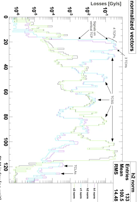
The values used for the centers of mass are the combinations of the signals on the four primary collimators (cf. Each of the 4 plots corresponds to the loss scenario (known before the calculation) given in the title of each plot. The results of the centers of mass perfectly match the type of each individual vector.
Each of the 4 plots corresponds to a scenario (known before the calculation) indicated in the title.
Choice of the algorithm
Various corrections were considered, such as subtracting the signal from the vertical collimator from the horizontal one, or stretching the variation interval. The implementation of the first method showed that a factor of approximately twice the vertical signal had to be subtracted to get a correct variation interval; but it created a pole for the function (h, v) 7→ (h−α ·v, v), i.e. the arbitrary stretch of the variational interval, which corresponds to the precedent method with no pole and a correction factor of higher value, led to the problem that some values of the mass centers are higher than one, in cases where the crosstalk between the two monitors is overestimated.
In the end, the choice was made to keep the centers of mass uncorrected, knowing that the horizontal/vertical would vary between -1 and -0.5.
Evaluation of the correctness of a decomposition
Averages are lower for SVD (better recomposition), and correct and incorrect are close to each other. The averages are lower with SVD (better recomposition), and regular and irregular are still too close to each other to allow good separation. For incorrect parses, 26 entries are above average (79% true negatives) and 7 below (21% false positives).
For the correct decomposition, there are 38 entries below the mean (54% . true positives) and 33 above (46% false negatives). for the incorrect breakdowns, 24 above (73% true negatives) and 9 below (27% false positives).

Application to LHC data
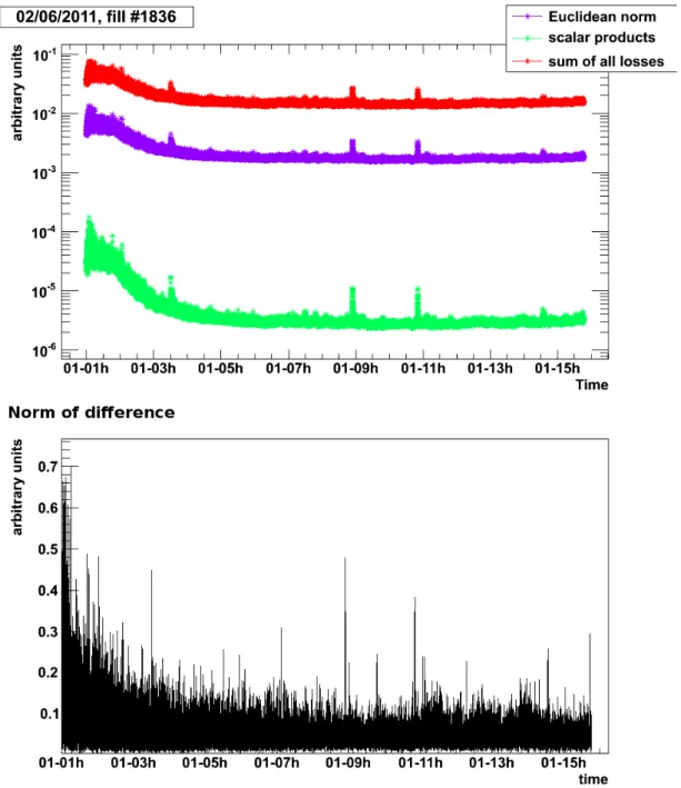
The first value calculated here is the rate of difference (subtraction) between the normalized vector representing losses in one second and the normalized vector representing losses in the previous second (cf. fig. 4.21):. Calculating the Euclidean norm of the vector is a good way to estimate the magnitude of the overall losses at the LHC (cf. fig. 4.21). In addition, the vector rate is several orders of magnitude higher than the "shape change" (cf. fig. 4.21).
So the scalar product is dominated by the effect of the norm and evolves like the norm.
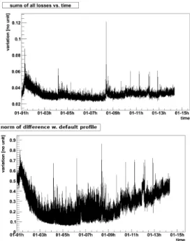
Default Loss Profile
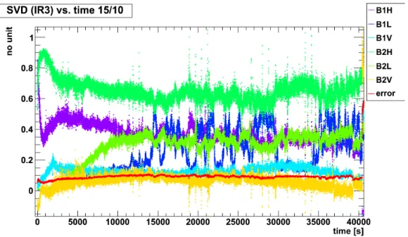
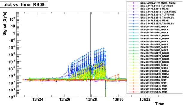
The work presented in this chapter focused on studying the time evolution of the signals from the Beam Loss Monitors during nominal operation. The point is to learn how the losses evolve; check where significant losses occur and which parts of the LHC are free of losses. It will also provide a better understanding of the behavior of the vectors and what information can be extracted from their time evolution.
TIME EVOLUTION
- Individual evolution of the signal of a BLM
- Evolution of the overall losses
- Conclusion
- Results of decomposition
It will describe the total loss in a similar way to the norm of the loss vector. It was performed by calculating the distribution of the difference between the signal of one BLM in one second and the previous second (cf. Figure 5.6). For the degree of precision of the loss measurement, the variations of the signal are Gaussian.
The norm of the difference also decreases in the first 3 hours; this is shown in more detail in fig.
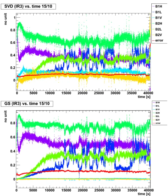
SPATIAL DECOMPOSITION
Examples of decomposition versus time
The error onxj, written asσxj, is the error on the BLM size. This is known: it is the standard deviation of each coordinate of the reference vector over all the loss maps that make up this vector. They are dominated by the error on the loss maps and are at least 3 orders of magnitude lower than the values of the factors, so they are not shown in the results.
All errors are less than 3 orders of magnitude or more of the values of the factors.
Validation of results
At the beginning of the filling, the total derivative is dominated by the derivative of Beam 1: the center of mass is positive. When the intensity derivative is dominated by beam 1 (CoM closer to 1), the decomposition is dominated by factors of beam 1 (CoM closer to 1). Bottom: correlation between the derivative of the intensity in beam 1 (Y-axis) and the SVD factor associated with B1H (X-axis).
For higher values of the factor, many more protons were lost (higher negative values of derivative).
Conclusion
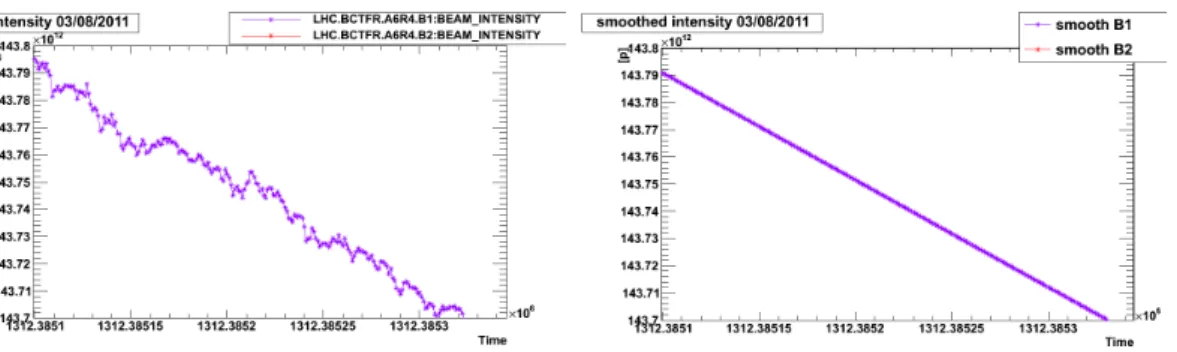
But during scraping the losses increase greatly; and the shape of the vector is then closer to the standard and the loss is better compounded. This shows that the error is an effective way to evaluate the quality of the recomposition. The reason for this is visible in the plot of the beam intensity versus time (cf. Fig. 6.15 center).
New reference vectors could be constructed for other scenarios, such as breaking the collimator hierarchy.
Introduction
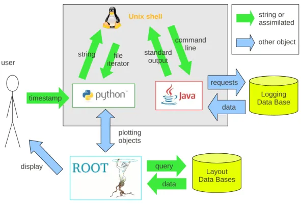
DATA ACCESS
Types of required data and corresponding databases
Loss thresholds are different from BLM to BLM, depending on the element they protect; they also vary depending on the 32 beam energy levels and LHC cycle phases. The actual thresholds used at the same time are stored in the databases, under a variable name similar to that of the loss: BLM_EXPERT_NAME:THRESH_RSXX where. The structure of the Layout database is that of a standard SQL database: several tables hold all related information in different columns.
Two identically behaved databases are used to store the values coming from the LHC's beam instruments.
Database Access Techniques
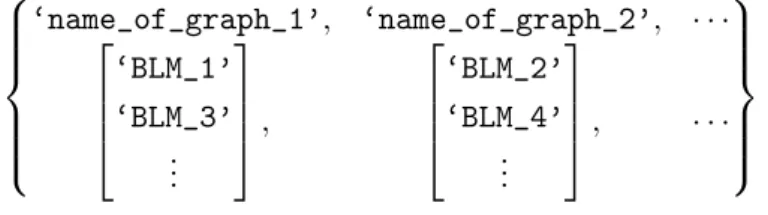
But once created, they are fixed: they do not follow the evolution of the variables in the database. Since not all variables are logged on the same time stamp (cf. § A.2.3), it was chosen to link each value to its time stamp, as this has already been done in the database. To link the list of values to the name of the variable, a mapping is performed thanks to a layout object.
The fact that all lists are the same length is guaranteed by the database structure.
Display
This is used as the X coordinate, where the Y coordinate is the second element of the 2-tuple. All this and creating the TLegend is done by the display.rainbowplot function. The format of the data recorded by this plot is as follows: the dual (pair) of base values is: (DCUM, value of the loss at the displayed timestamp).
The plot time is an important value displayed in the title of the plot.
The wrapping module: analysis
This list (ordered by DCUM) is downloaded from one of the layout databases called MTF. The name of the graph describes the criteria validated by the BLMs on the list, e.g. The display of the signal from the BPMs requires a similar process to the BLMs.
The mapping of the value with the name and position must be done after the data query.
Conclusion
CROSS-CHECKS
Any monitor, sensitive to a secondary shower of mixed particles originating from protons lost in the LHC. Short parts of the accelerator where the majority of the beam operations take place (collision, acceleration, cleaning, measurements..) by opposition to the arcs, where the beam is carried. Predefined integration interval used as a sliding integration window by the BLM electronics to evaluate the duration of a beam loss (cf.
Zamantzas, "The Real-Time Data Analysis and Decision System for Particle Flux Detection in LHC Accelerator at CERN", CERN-thesis-2006-037.