in Type II GaAs/AlAs Structures

The macro-photoluminescence experiments that led to the discovery of quantum dot formation in the GaAs/AlAs bilayer are described. In the second section, the advantages of quantum dots formed in GaAs/AlAs type II bilayer over many other systems in exciton complex studies are given.

What are exciton complexes?

The advantages of GaAs QDs formed in a type II structure

Harmonic confining potential

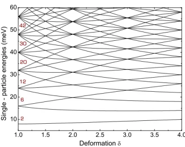
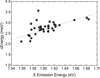
An example of the dimensions and width of the lateral potential for a typical point is shown in Fig. 2.4. The dashed vertical line illustrates the limit of the quantum dot dimension that can be deduced from experiment.

Figure 2.2: Single particle states of a two-dimensional anisotropic harmonic oscil- oscil-lator as a function of deformation δ > 1

Shell degeneracy

Fig.2.5 illustrates this effect when the restriction is increased from 3D system (bulk) materials to 0D systems (quantum dots). In the quantum dot, the density of states becomes discrete and is similar to set of δ-functions.

Exciton in a quantum dot

Exciton binding energy

In general, several methods have been applied to evaluate the exciton binding energy in a quantum dot of defined size. In the case of the investigated quantum dot, the exciton binding energy is estimated to be about a dozen meV.

Modification of energy levels in a magnetic field

Quantum dot exciton in a magnetic field
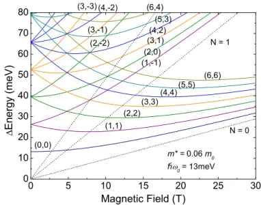
Carriers in a harmonic potential in a high magnetic field
Energy structure
TEM images

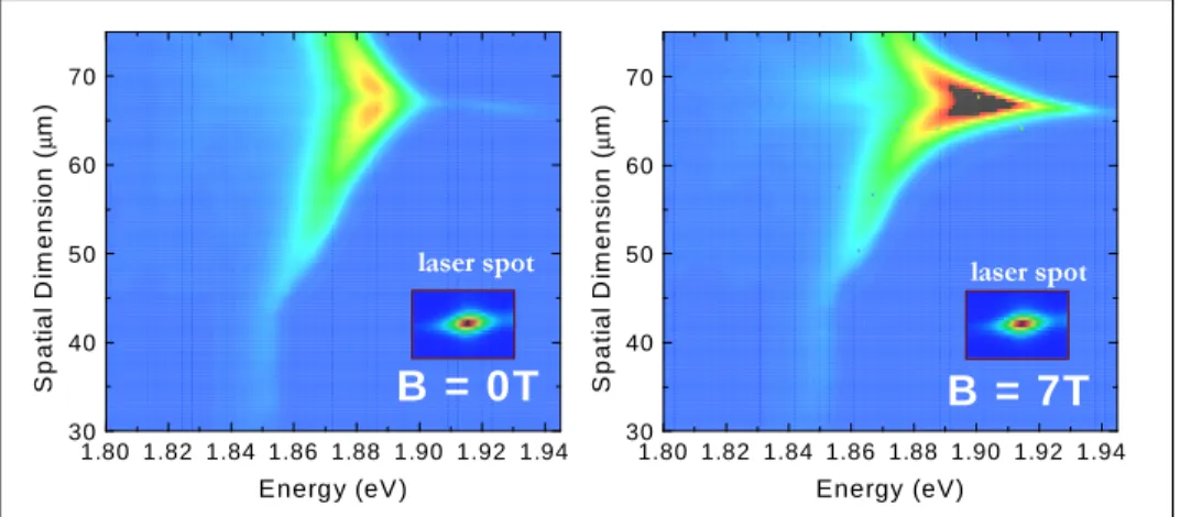
The diamagnetic shift magnitude is determined by the spatial dimensions of the exciton wave function in the direction perpendicular to the magnetic field. The development of the energy spectrum in the increasing magnetic field is illustrated in Fig.2.6.

Figure 2.6: Fock - Darwin energy levels at magnetic field. Dotted lines correspond to the first three Landau levels.

GaAs quantum dots

Energy structure
KFM images
Excitation sources
Detection

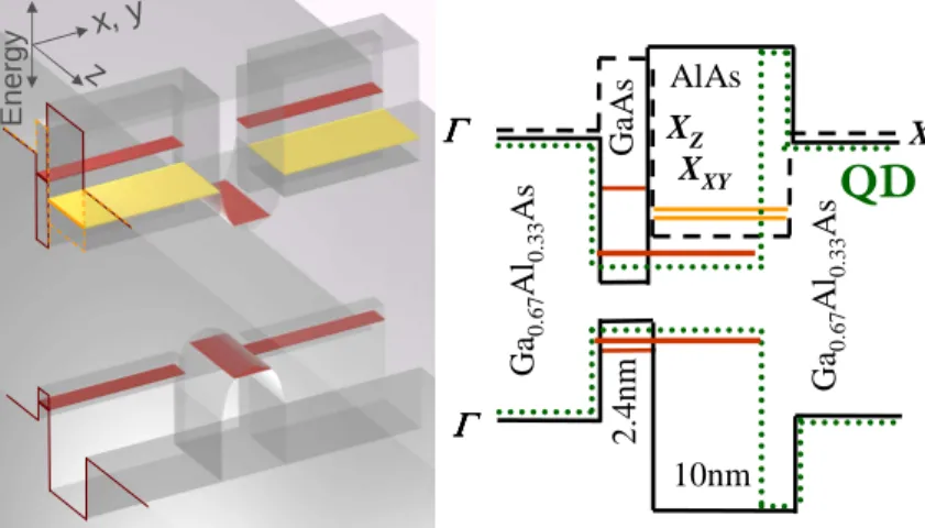
The three-dimensional image illustrates the symmetry and shape of the point potential (harmonic type) in the plane of the quantum well layers. The positions of the first electronic levels in the quantum well and dot are marked as the colored layers.

Figure 3.3: Potential distribution through the quantum dot formed in the GaAs/AlAs type II double quantum well structure is marked schematically on the potential distribution of double quantum well structure (compare with Fig.3.1 a);

Macro-photoluminescence

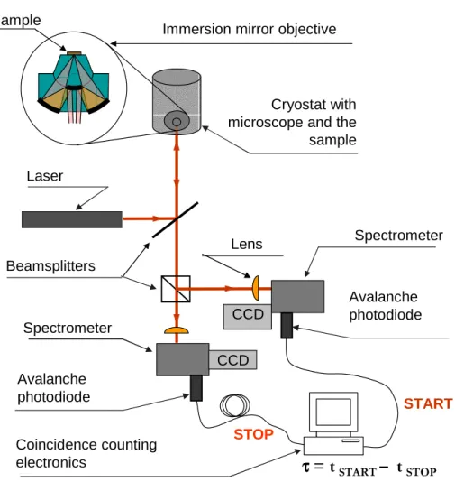
Standard PL setup

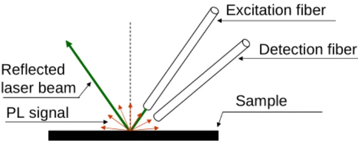
Optical fiber system

This ensures that most of the laser light is reflected from the sample surface away from the collection fiber. Nevertheless, due to the large value of the refractive index of GaAs (n = 3.3), the incident light enters the sample almost parallel to the direction of the magnetic field.

Figure 4.2: Geometry of a two-fiber system to minimize the gathered laser light.

Micro-photoluminescence

Variable temperature experiments
Micro-PL mapping
PL imaging
High magnetic field setup

The scanning of the sample surface was performed by placing a thick parallel plate in front of the microscope objective. The position of the laser beam on the sample surface was changed by rotation of the plate.

Generation of magnetic fields

The connection of the laser and the spectrometer to the optical fiber outputs are similar as illustrated in Fig.4.3. The experimental setup was available at the High Magnetic Field Laboratory, CNRS in Grenoble, France.

Time resolved experiments

Photon correlation

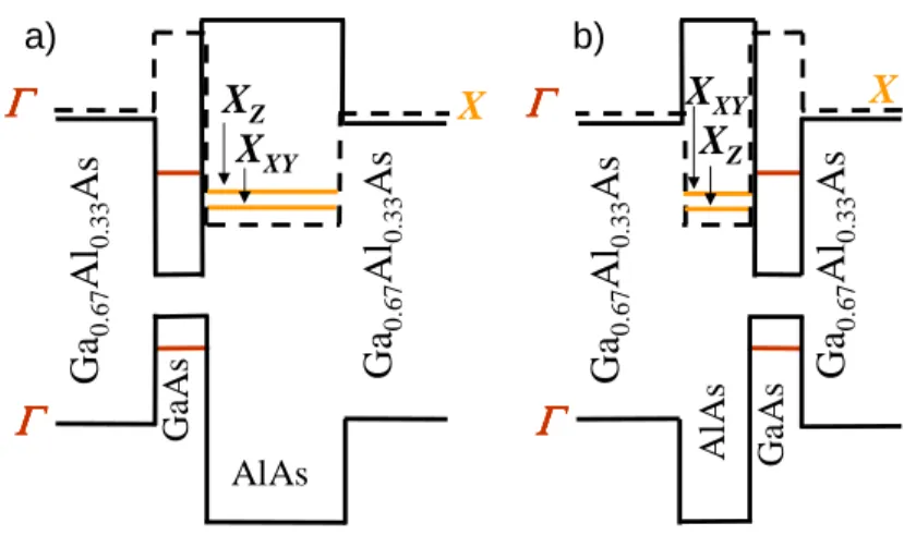
Twiss, “The Question of Correlation Between Photons in Coherent Light Beams.” Nature (London), vol. This is in contrast to the GaAs/AlAs type II pseudodirected structure, in which the lowest electronic state in the AlAs cavity is of XZ and XXY symmetry.

Quantum-dot-like luminescence

It is very likely that there is another type of "localization trap" in the active part of the sample that leads to the appearance of the observed sharp emission lines. In order to explain the occurrence of such "deep traps" in the investigated sample, the possibility of effective diffusion of Ga into the AlAs layer during the MBE growth of the structure is noted. The temperature-dependent macrophotoluminescence experiment made it possible to conclude that the origin of the sharp emission lines is the result of highly localized states present in the structure, most likely quantum dots.

Figure 5.3: Photoluminescence spectra measured for different temperatures be- be-tween 4.7K and 104K on indirect type sample [4].

Characteristic lifetimes in the system

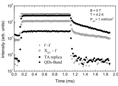
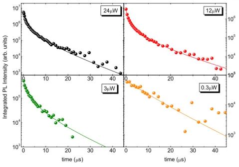
The proposed scenario implies that the diffusion process of the long-lived carriers is an important element in understanding the observed phenomena and should be reflected in the kinetics of the emission. They are shorter than 10 ns, which in this case is the limit of the experimental setup. The decay time of the quantum dot luminescence appears to be within the µs range.

Figure 5.5: Time-resolved decay measured for different transitions with a time window of ∆t = 20µs

Diffusion

This was achieved by reducing the size of the excitation spot in the µ-PL technique. The dot is therefore populated even from large distances from the excitation site to the dot. This is possible when an impurity is present near the dot (or some other source of possible charge fluctuation).

Figure 5.7: Spectrally resolved µ-PL images taken for pseudo-direct transition.

Zero and first order excitonic complexes - X, X* and XX

Effects of the confining potential and quantum dot composition 60

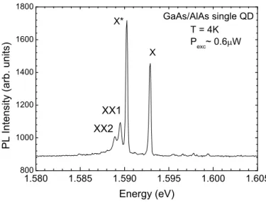
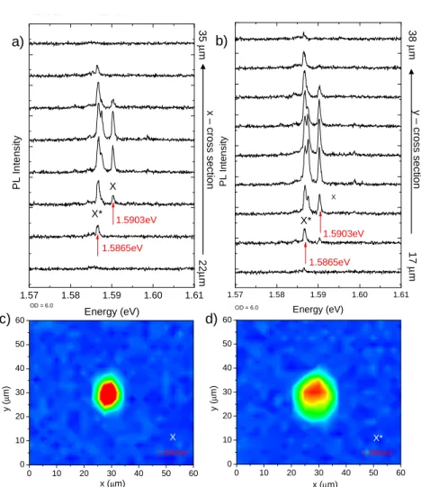
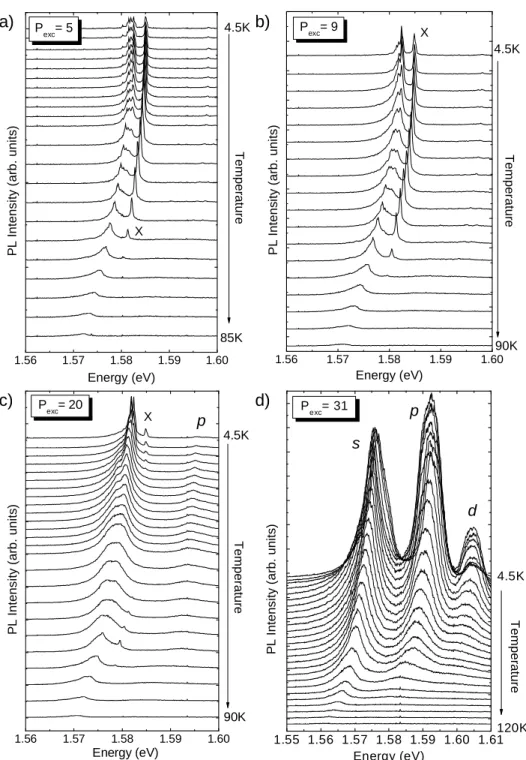
No dependence between the X emission energy and the size of the lateral confinement potential was found. The appearance of emission lines: X, then X* and XX1 in the PL spectra is observed with increasing excitation power. With increasing excitation power, we observe a linear growth of the X emission and super linear for more complex structures.

Figure 6.5: X* binding energy for different quantum dots: the energy difference between X and X* emission versus X emission energy.

Charged and empty quantum dots

Fig.6.9 illustrates the emission energy shift, with respect to the excitonic emission, in the whole range of excitation powers up to the limit where the X-emission disappears. Fig.6.10 illustrates the excitation power evolution of different quantum dots than those presented in Fig.6.7 in the same range of excitation powers. It is observed that the X* emission is the simplest excitation in the case of the lowest excitation power.

Magnetic field effect

µ-magneto-PL spectra of X, X* and XX excitonic states
Diamagnetic shift
g-factor
Thermalization effects
X as bound state
Mapping experiment
Hidden symmetry properties of the system

The excitation power evolution of the emission spectra for this particular dot is illustrated in Fig. 6.10. The magnetic field evolution of the single quantum dot emission measured at low excitation power. The observed population inversion of the Zeeman splitting levels in the quantum dots is an intriguing effect.

Figure 6.11: µ-PL spectra of the single quantum dot scanned in the a) x- and b)y- directions

Many-body type effects

Band gap renormalisation

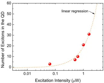
Excitation intensity (W) linear regression. Figure 7.7: Changes in the number of excitons in a dot with increased excitation intensity, evaluated for the quantum dot from Figure 7.2a). The estimate of the excitation intensity for the number of carriers in the dot is approximate in this case. It is assumed that the number of excitons in a quantum dot increases linearly with the excitation power.

Figure 7.7: The changes of number of excitons in the dot with increased excitation intensity evaluated for the quantum dot from Fig.7.2a).

Confining magnetic field - Fock-Darwin diagram

Conclusions from the Fock - Darwin model

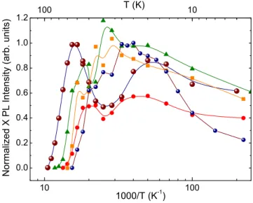
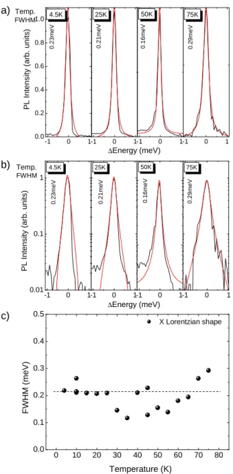
Therefore, apart from the interactions between carriers at multiple levels (as discussed in section 7.1.2), the effects of interactions of carriers in the same shell are clearly visible when the shell is completely filled. Within the experimental resolution, the width of the X-line is stable up to 70K when the emission line is extinguished, as discussed in Section 8.4. As the emission intensity decreases, the recovery of the X emission line is observed around 70K in Figure 8.3 c).

Figure 8.1: Typical µ-PL spectra of four different quantum dots (a - d) excited with small excitation power to observe single excitonic emission lines.

Band-gap shrinkage

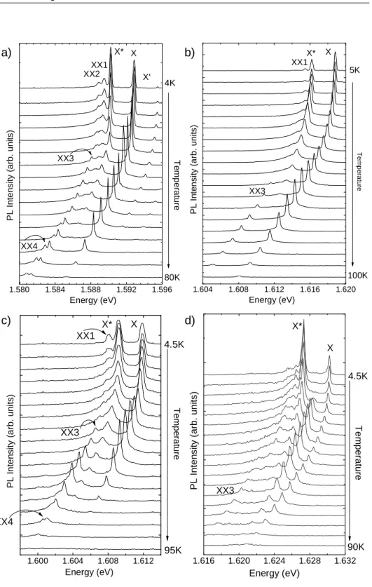
The effects of the temperature increase on the emission properties are: the quenching of PL intensity, emission energy shift, appearance of low energy emission lines and small line broadening effects. The emissions in each image are normalized in intensity to compare the change of line shape with increasing temperature. The temperature-induced energy shift of the emission lines is well described by the band gap energy shift in the Einstein model due to the change of atomic constants and electron-phonon interaction.

Figure 8.3: The temperature evolution of the emission spectra for the same quan- quan-tum dot taken with different excitation powers a) P exc = 5, b) P exc = 9, c) P exc = 20 and c) P exc = 31

Role of radiative and non-radiative processes

Thermally activated emission

One possible scenario is that this recombination involves a number of excited states in the initial and final states of the recombining carriers. This splitting of the final states is most likely assigned to the hole remaining in the excited p-shell state after recombination, since the energy difference between hole shells is smaller (~1meV) than that of electrons (~7meV). Therefore, the XX3 and XX4 emissions are likely due to positively charged exciton and/or biexciton recombination in the excited states.

Figure 8.8: Integrated emission intensity of the single exciton emission line, X, for several quantum dots.

Line broadening effects

This may be due to the weak interaction of electrons with acoustic phonons in the case of the investigated quantum dots. Cardona, “Temperature dependence of critical point shifts and broadenings in GaAs,” Phys. Forchel, “Temperature dependence of the homogeneous exciton linewidth in self-assembled In0.60Ga0.40As/GaAs quantum dots,” Phys.

Figure 8.10: a) Examples of a Lorentzian fit to single X emission lines at temper- temper-atures 4.2K (a), 25K (b), 50K (c) and 75K (d) for the quantum dot which emission spectrum is illustrated in Fig.8.1a)

Spectrally and temporally resolved emission from a single dot

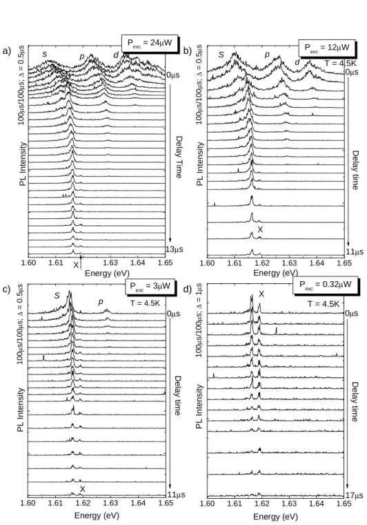
The excitation power in the laser pulse is constant for all measurements, and the changes in time of the spectra are tracked for different temperatures in the grating. Similar to the experiment performed for different excitation powers, a subsequent depletion of the dot states is observed. The time evolution of photoluminescence spectra of a single quantum dot revealed very long decay times on the order of tens of µs.

Figure 9.2: Time resolved photoluminescence spectra of single GaAs quantum dot for different powers of the excitation pulse at 4.2K.

Diffusion of indirect excitons

The temporal evolution of the emission from the quantum dot reflects the dynamics of carriers in the 2D quantum well system. Section 10.1 discusses the differences in the emission spectra under resonant and non-resonant excitation. Fig. 10.2 illustrates the comparison of the excitation power evolution of the same quantum dot spectra under quasi-resonant and non-resonant excitation.

Figure 9.6: Transients measured for the same quantum dot for different excitation powers (the same as illustrated in Fig.9.4a) fitted with eq.9.3, see text for details.

General characteristics of the photon correlation experiment

Second order correlation function

The excitation power-dependent emission spectra of a single quantum dot taken under quasi-resonant and non-resonant excitation revealed that in the case of quasi-resonant excitation, the sharp line emission is much pronounced in a wide range of excitation. forces. When the dot is excited above the band gap, a rapid appearance of broad bands is observed with increasing excitation power, indicating stronger interactions of carriers with the dot environment, leading to broadening of the emission lines. In all experimental results presented below, the exponential law according to Equation 10.2 was fitted to the exponential decay times.

Exciton in a quantum dot as a single photon source

The sharp anti-bonding peak exactly at zero lag time is a typical feature of autocorrelation histograms. The width of the anti-bounce dip decreases as the excitation intensity is increased (compare with Fig.10.7). The anti-bonding dips exactly at zero delay time in autocorrelation photon histograms show that only one configuration of carriers exists in the quantum dot at a given time.

Charge fluctuation in a quantum dot - single carrier capture or

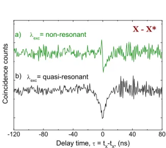
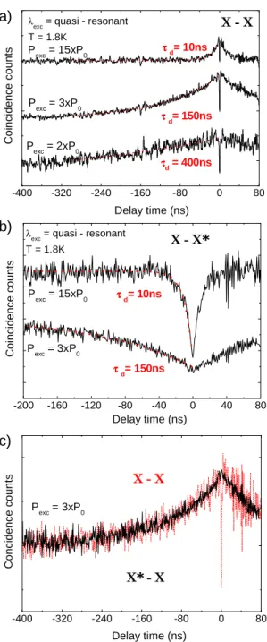
The strong clustering at τ < 0 indicates that the single-carrier trapping process is very effective and the shape of the histogram resembles that of cascade emissions (compare Fig. 10.12). The process can be well described by the rate equations according to the population diagram illustrated in Fig.10.6a). The model involving the rate equations to fit the histogram illustrated in Fig.10.5a) was made in Ref.[19] and will not be repeated here. If the process is suppressed, for example by resonant excitation, markedly different effects are observed. Fig.10.5b) illustrates the X - X* cross-photon correlation histogram obtained under resonant excitation.

Figure 10.5: X-X* cross-correlation histogram taken under a) non-resonant and b) quasi-resonant excitation.

Charge fluctuation process under resonant excitation

In the case of quasi-resonant excitation, the two stable states of the dot are the neutral state and the special X*-type charged state. Similarly, increasing the number of point carriers significantly shortens the observed times. A comparison of X-X and X-X* autocorrelation histograms obtained for the same excitation power and excitation energy is illustrated in Fig.10.7c).

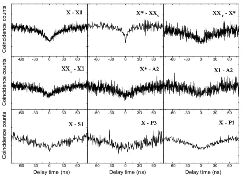
Figure 10.7: a) X - X auto-correlation histograms and b) X - X* cross-correlation histograms for different excitation powers at quasi-resonant excitation, different for a) and b) (see text for details)

Neutral and charged families of quantum dot states

In the picture, the X-X* histogram is inverted and both are normalized to the same number of counts. This confirms that the charge state variation in the spot occurs between the two possible (neutral and one type of charged) configurations of carriers. It can therefore be concluded that, in the case of the quantum dot studied, only one type of charged states is observed.

Figure 10.8: The set of cross-photon histograms of correlated counts as a function of time interval τ = τ ST OP − τ ST ART between photon registration events in start and stop detectors, tuned to indicated transitions (start-stop order)

Charge variation on the ”macro” time scale

In the case of the upper graph, the spectra were recorded while the position of the laser spot on the sample was slightly changed. In the case of the bottom plot, the excitation intensity varied to a very small degree. In the present experiment, by slightly scanning the spot with the laser beam or with small variations of the excitation power under quasi-resonant excitation, it was possible to switch between the two spectra illustrated in Fig.10.9.

Figure 10.9: The very long time blinking effect visible in the micro-PL spectrum of the single GaAs/AlAs quantum dot (different dot than the one whose emission spectrum is illustrated in Fig.10.1) at moderate excitation power and quasi-resonant excitation

Cascaded multiexcitonic emission

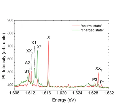
Neutral cascades

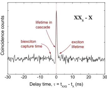
The illustrated spectrum is mainly due to the recombination of the neutral configuration of carriers in the dot. The spectrum of the quantum dot, taken at a relatively low excitation power for the most 'neutral' configuration of carriers in the average time of spectrum accumulation, is illustrated in Figure 10.11. The typical fingerprint of the cascaded emission [15, 23] from the quantum dot is the shape of the histogram observed for exciton (X) and biexciton singlet (XXS) states.

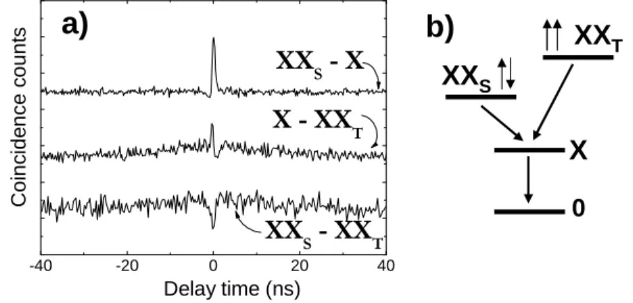
Figure 10.12: X-XX cross-correlation histogram illustrating that the two states are connected into a cascade with XX being the initial state.

Biexciton triplet state

In the experiment, a small magnetic field of 0.5T was applied to better resolve the polarization of the emission lines. This extremely long time was assigned to the change in the surroundings of the quantum dot. The experimental results that strongly suggest that the observed oscillations are not caused by the variation of the excitation power during the measurements are: .. the spectra are stable and very well reproducible in a given magnetic field .. the magnetic field of the observed maximum and minimum versus the number complete was found to be a linear function∗, which is illustrated in Fig.12.2 c).