Motivation
In the case of varying coefficients and various space dimensions, the associated stabilization problem is addressed in [AB99, AB02, ABL11b]. Then we derive a (partial) solution to the two open questions raised above for parabolic systems. We also prove that similar controllability results hold for the boundary control problems (1.2) and (1.4), which partially answers the second question.
In one spatial dimension in particular, the geometric conditions reduce to a non-emptiness state and are therefore optimal even for parabolic systems. At the end of the present introduction, we present our main results for wave/heat/Schr¨odinger-type systems. In Section 2, we present an abstract setting adapted to second-order (in-time) control problems.
Finally, in Section 6, we come back to the applications for wave/heat/Shr¨odinger-type systems. The first author would like to thank the Fondation des Sciences Math´ematiques de Paris, the organizers of the IHP trimester on control of PDEs and the Laboratoire MAPMO for their support.
Main results
Note that in the case kurc= Id and a= 0, the best constantλ0 is the smallest value of the Laplace operator on Ω with Dirichlet boundary conditions. In the work [BLR92], the authors prove this observation inequality with all these boundary conditions (all consistent with the Melrose-Sj¨ostrand propagation theorem of singularities). According to the operator property A, the injection Hk֒→Hk−1 is dense and compact for anyk∈Z.
In the following, we shall, as in [AB03], make use of the different energy levels. For System (2.3), now studied inH1, we only need to observe the state of the first component, i.e. u1, u′1), and thus define an observation operator B∗ ∈ L(H2×H, Y), where Y is a Hilbert space that stands for our observation space. The operator B∗ is an admissible observation for Note that only the energy level of the second component v2 is needed in this admissibility estimate.
We can now state our main result, viz. 2.7) Note that the constants p∗ and T∗ can be given explicitly with respect to different parameters of the system. The internal control result from Theorem 1.3 is then a direct consequence of HUM, since assumptions (A1)-(A3) are fulfilled in this application. As a consequence of the admissible inequality (2.6), the system (2.8) is well placed in H0 in terms of transposition solutions.
In this setting, the boundary check result of Theorem 1.3 is a direct consequence of the HUM and Theorem 2.2, since Assumptions (A1)-(A3) are met in this application.
Some remarks
If the operatorB is bounded, we proved in [ABL11b] (under similar assumptions) a polynomial decomposition result for the energy E1(U(t)) of the system. The observability estimates for a single right-sided equation that we prove here (Lemma 3.3) also improve the results of [ABL11b] in the restricted B case. The main advantage is that it provides a systematic method for internal and boundary controllability problems for a large class of second-order time equations.
We only need to check if an observability inequality is known for a single equation, and the results can be transferred directly to systems. However, we have to make several assumptions here: symmetry of the system, coercivity of the elliptic operator, smallness of the coupling coefficients, large control time. We do not know exactly which assumptions are really necessary and which are unnecessary.
Finally, note that these exact controllability results for second-order abstract hyperbolic equations yield zero controllability results for heat- or Schr¨odinger-type systems in the abstract setting as well. However, for the sake of clarity, we do not state these results in an abstract setting, but only for heating or Schr¨odinger systems (see Sections 6.2 and 6.3). In the following sections, when we prove Lemma 2.1 and Theorem 2.2, we will use two different energy levels.
Note that this system has a unique solution (w1, w2), since the AP operator is constrictive, which also satisfies w′′1+Aw1+P w2= 0,. Now, the idea is that, for sufficiently small p+/λ0, the energy e0 of v2 is almost equivalent to e1. The last two identities are technical estimates, used at several points in the proof of the observation inequality.
Two key lemmata
Proof of Lemma 2.1: admissibility
Proof of an observability inequality with a right hand-side
Note that the important feature is that the observability constants KB and KP do not depend on the timeT asT here. It is linked to the invariance properties of the system with respect to translation over time. Such observable inequalities are proved by multiplication techniques for the wave equation or the plate equation in [AB02, AB03, ABL11a].
Here, proving (3.14) and (3.15) as a consequence of the associated observation inequality for the free equation (Assumption (A3)) and an admissibility assumption (A1) has several advantages. In particular, we can use as a black box the different observation inequalities obtained for different equations (eg [BLR88, BLR92] for waves) and thus obtain results with optimal geometrical conditions. However, for the sake of completeness, we also prove Lemma 3.3 in a simple case for the wave equation directly in Appendix 7, with optimal geometric conditions.
The proof of (3.15) is simpler, since the observation operator ΠP is bounded (and we therefore do not need an admissibility assumption). To prove the first inequality of (3.14), we first split a solution of ϕ′′+Aϕ=f into ϕ=φ+ψ, where φ and ψ satisfy. and we give upper bounds for both integrals on the right-hand side. 3.19). To get the observation on ϕ instead of ψ on the right-hand side, we write 3.20) Then, using the admissibility assumption (A1) we get forφ.
Since the equation ϕ′′+Aϕ=f is invariant under time translations, the last inequality gives, for allT2≥T1+TB∗,. In each of these integrals, the time interval is greater than TB∗, so we can use (3.22). In this section, we will often use the notation A.B, which means that there exists a universal numerical constant C >0 (depending on none of the parameters of the system) such that A≤CB.
In this section, we give the connection between v1 and v2 that we will use in the following.
A first series of estimates
A second series of estimates
Using the two estimates of this lemma, together with the right-hand observability inequality for the operator ΠP, given in Lemma 3.3, we can now prove the following lemma. Integrating this inequality on the interval (0, T) and using Identity (3.4) along with the conservation of energy E1(W), we obtain. Now using assumption (A2) and integrating the last inequality on the interval (0, T), this yields >0 for all ε.
End of the proof of Theorem 2.2
Now it remains to check whether these coefficients are positive for a suitable choice of ε(small) and T (large). Thus, for this choice of p+, ε sufficiently small and T sufficiently large, we obtain from (4.18) the existence of a constant C > 0 such that. In this section we prove that the observability inequality of Theorem 2.2 (or equivalent Theorem 4.7) implies the verifiability results of Theorem 2.3 and 2.4.
This is done in a classical way using the Hilbert Uniqueness Method (see [Lio88]), which we will follow here. Note that, as in the concrete setting, it also preserves the space H1×H2×H×H1 over time once P ∈ L(H1). Note that a direct application of the HUM, at the energy level H1×H×H×H−1 for the adjunct variable V, would yield a controllability result in H×H−1×H1×H with a controlBf ∈L2(0 , T;H−1) (and we should assume that B∈ L(Y, H−1)).
Then for all T > T∗ (given by Proposition 4.7) the solution Z for some constant C >1 satisfies the estimates. We will also use the following lemma to prove Theorem 2.3 with HUM. By definition, the linear formLi is continuous on X and, according to (5.2), the bilinear form is continuous and coercive on X × X as soon as T > T∗.
The Lax-Milgram theorem then ensures for T > T∗ the existence (and uniqueness) of ZT such that.
The linear form Lis is continuous on X and, by the admissibility inequality (2.6) and the observability inequality (2.7), the bilinear form a is both continuous and compelling on X × X as soon as T > T∗. In this section, we explain how Theorem 1.3 and Corollaries 1.4 and 1.5 can be derived from the abstract results. We only need to explain how the situation of this statement can be placed in the abstract setting.
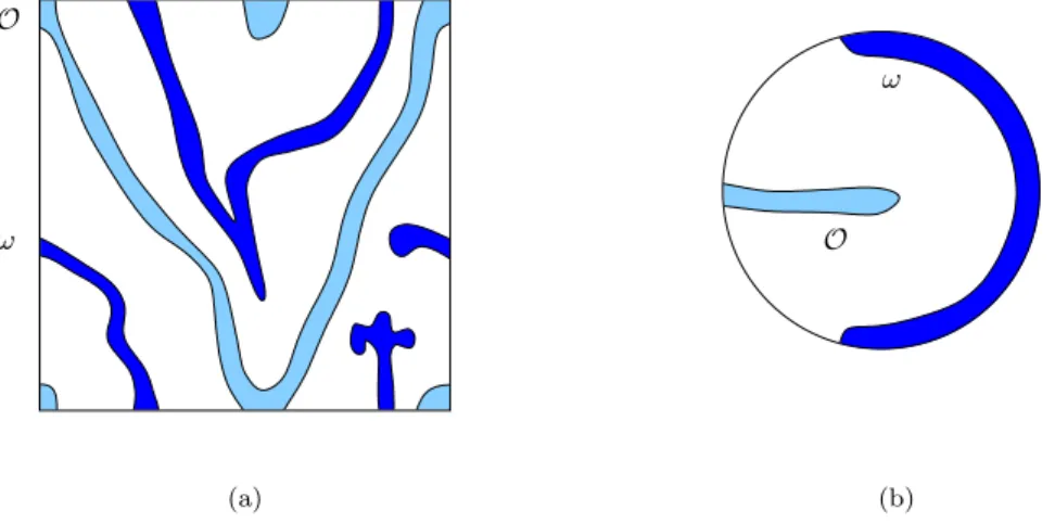
According to Assumption 1.2-(ii), ωp satisfies the GCC, so that the observability inequality of [BLR88, BLR92] directly implies the second part of Assumption (A3). Finally, according to assumption 1.2-(iii), ωb satisfies the GCC, so that the observability inequality of [BLR88, BLR92] directly implies the first part of assumption (A3). All assumptions of Theorem 2.3 are then met, so that this implies Theorem 1.3 in the case of internal control.
Finally, by Assumption 1.2-(iii), Γb satisfies GCC∂, so the observability inequality [BLR92] directly implies the first part of Assumption (A3). All the assumptions of Theorem 2.4 are then satisfied, thus implying Theorem 1.3 in the case of limit control. Note that one could take the initial data in less regular spaces, provided the coefficients a, p are smooth enough.
The proof of Corollary 1.5 is the same as that of Corollary 1.4, except that the Schr¨odinger equation does not enjoy smooth properties. In this section we provide a direct proof of Lemma 3.3 for a wave equation in a very simple setting. In particular, it shows that the observability inequality for equations with a right-hand side are indeed the natural energy estimates in the spaces we consider.
If ρ /∈Char(P), then P is elliptic of the second order at ρ and the first equation of (7.3) yields datv ∈H2 microlocally at ρ. H¨ormander's theorem on the propagation of singularities [Tay81, Chapter 6, Theorem 2.1] (see also [H¨or94, Theorem 26.1.1]) yields that v∈H1 microlocally on ρ since v satisfies P v∈L2. Spectral inequalities for non-self-adjoint elliptic operators and application to the zero controllability of parabolic systems.