HAL Id: hal-00294247
https://hal.archives-ouvertes.fr/hal-00294247
Submitted on 9 Jul 2008
HAL
is a multi-disciplinary open access archive for the deposit and dissemination of sci- entific research documents, whether they are pub- lished or not. The documents may come from teaching and research institutions in France or
L’archive ouverte pluridisciplinaire
HAL, estdestinée au dépôt et à la diffusion de documents scientifiques de niveau recherche, publiés ou non, émanant des établissements d’enseignement et de recherche français ou étrangers, des laboratoires
Interaction with a field: a simple integrable model with backreaction
Amaury Mouchet
To cite this version:
Amaury Mouchet. Interaction with a field: a simple integrable model with backreaction. European
Journal of Physics, European Physical Society, 2008, 29, pp.1033-1050. �hal-00294247�
Interaction with a field: a simple integrable model with backreaction
Amaury Mouchet
Laboratoire de Math´ematiques et Physique Th´eorique, Universit´e Fran¸cois Rabelais de Tours — cnrs (umr 6083),
F´ed´eration Denis Poisson,
Parc de Grandmont 37200 Tours, France.
mouchet@phys.univ-tours.fr July 9, 2008
PACS: 46.40.Cd, 46.40.Ff, 42.50.Ct, 03.65.Yz.
Abstract
The classical model of an oscillator linearly coupled to a string cap- tures, for a low price in technique, many general features of more realistic models for describing a particle interacting with a field or an atom in a electromagnetic cavity. The scattering matrix and the asymptotic in and out waves on the string can be computed exactly and the phenomenon of resonant scattering can be introduced in the simplest way. The dissipa- tion induced by the coupling of the oscillator to the string can be studied completely. In the case of a d’Alembert string, the backreaction leads to an Abraham-Lorentz-Dirac-like equation. In the case of a Klein-Gordon string, one can see explicitely how radiation governs the (meta)stability of the (quasi)bounded mode.
1 Introduction
Getting back to the spirit of thexixthcentury — when purely mechanical mod- els were ubiquitous even for understanding systems involving electromagnetic fields — this paper discusses a simple model of an oscillator coupled to a string that presents a host of interesting features in a very accessible way. It will be presented in detail in § 2 (see figure 1). Even though the required technical background is on an upper undergraduate/early graduate level, if one remains within a classical (i.e. non-quantum) context, this model encapsulates many relevant features of physical interest which can be found in more realistic mod- els, for instance when considering the interaction of an atom (the oscillator) with light (the string).
First (§3), when the string is infinite, it allows one to gain insight into (or to discover for the first time in academic studies) the scattering of waves by a dynamical system. It provides the opportunity to introduce some of the ingre- dients of scattering theory: when dealing with a one-dimensional mechanical
system, the notion of asymptotic states (the so-called “in” and “out” states) is made as simple as possible and the S matrix takes a particular simple form.
Unlike the transmission of light in a Fabry-Perot interferometer, the resonant scattering appears here explicitly in connection with the familiar resonance phe- nomenon of a forced oscillator and we can also understand how the motion of the oscillator affects in return the external excitation.
Second (§ 4), from the point of view of the oscillator, this model consti- tutes the most elementary example of radiation. It shows concretely how an interaction not only induces a shift in the natural frequency of the oscillator (this can already be seen when only two degrees of freedom are coupled) but also that the coupling to a large number of degrees of freedom (the string being seen as a large collection of oscillators) induces a friction term for the oscillator, although no dissipation exists in the system as a whole (for an electric analo- gous phenomenon see§ 22.6 of Feynman et al., 1970; Krivine & Lesne, 2003).
Indeed, as far as I know, there are very few places where this model is dis- cussed and always in the specialised literature with a d’Alembert string (Sollfrey
& Goertzel, 1951; Dekker, 1985). Some of its variants (Stevens, 1961; Ru- bin, 1963; Yurke, 1984; Dekker, 1984; Yurke, 1986) are introduced precisely for studying dissipation at a quantum level. As we will see, a Klein-Gordon string allows to keep one discrete mode (a bounded state) without dissolving it in the continuous spectrum of the string and therefore allows to mimic the interaction of a field with a stable particle, not just a metastable one. This model is parti- cularly relevant to see how backreaction works: For instance, for a d’Alembert string, the oscillator is governed by an Abraham-Lorentz-Dirac-like equation.
Besides, we will be able to illustrate precisely the deep connection between the resonance and the poles of theSmatrix (a major feature in high energy particle physics and in condensed matter physics).
Before we give some guidelines for further developments in the conclusion (§6), we will complete our classical study in§5 by the detailed diagonalization of the Hamiltonian and the discussion of the completeness of the basis of modes that are used to described the dynamics. This will be the occasion to sketch the finite size effects if one wants to use this model for describing an atom placed in a cavity. This study also prepares the ground for the quantization which will be proposed in a future paper.
2 The spring-string model
2.1 Description of the model
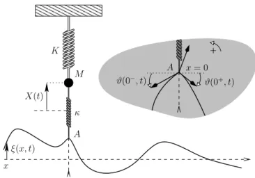
A very thin homogeneous string of linear mass µ0 is considered to have only transverse displacements in one direction. At equilibrium it forms a straight line along the x-axis with the uniform tensionT0 (we will never take into account the effects of gravity). The string is coupled to a system of mass M with one degree of freedom connected to a fixed support with a massless spring of stiffness K (see figure 1). The coupling is modelised by a second massless spring of stiffnessκattached to the string at the massless pointAatx= 0. All the vibrations will be considered within the harmonic approximation of small amplitudes. We will denote by ξ(x, t) the transverse displacement at timet of the string element located at x at equilibrium. The displacement of M with
+ K
M
A κ
x ξ(x, t)
X(t)
A x= 0 ϑ(0+, t) ϑ(0−, t)
Figure 1: Model of a harmonic oscillator coupled to a string via a massless spring. The long-dashed lines refer to the equilibrium positions of the string and the oscillator. The inset shows the three forces that cancel at the massless attachment point A (x= 0): the left and right tensions of the string and the elastic force of the coupling spring.
respect to its equilibrium position will be denoted byX(t).
2.2 Equations of motion
The equation of motion of the oscillator is Md2X
dt2 +MΩ20X =−κ(X−ξ0) (1a) where ξ0(t)def=ξ(0, t) is the displacement ofA and Ω0
def=p
K/M is the harmonic frequency of the free oscillator. Forx6= 0,ξfulfills the one-dimensional d’Alem- bert equation
∂2ξ
∂x2 − 1 c2
∂2ξ
∂t2 = 0 (1b)
where the wave velocity on the string is given bycdef=p
T0/µ0. The derivation of (1b) is a major step in every introductory course on waves (Crawford, 1968,
§2.2, for instance). Less common is perhaps the refinement of sticking the string to a “mattress” (see figure 2) made ofnmassless springs per unit length along thex-axis, each of them having a stiffnessκ. The restoring force per unit length due to the mattress,−nκξ, turns the d’Alembert equation into a Klein-Gordon equation
∂2ξ
∂x2 − 1 c2
∂2ξ
∂t2 −ω02
c2 ξ= 0, (x6= 0) (1b’) where ω0
def=cp
nκ/T0. This equation governs also the propagation of the elec- tromagnetic field in a rectangular waveguide (Feynman et al., 1970, chap. 24) and is also the relativistic equation of a quantum particle of mass ~ω0/c2, c being the velocity of light in the vacuum.
Figure 2: A mechanical model that leads to a Klein-Gordon equation: the string is attached to an elastic support that can be seen as a tight collection of massless springs uniformly distributed per unit length along the string. For another mechanical example, see (Crawford, 1968,§3.5).
Since the attachment point A is massless, the sum of the three forces ap- plied to it vanishes as depicted in the inset of figure 1. To first order in the slope ϑ(x, t) = ∂ξ/∂x(x, t), the transverse component of the right tension ap- plied to A is given by T0ϑ(0+, t) the limit when x → 0 keeping x > 0. On the other side, the transverse component of the left tension is−T0ϑ(0−, t). The restoring force of the coupling string corresponds to the opposite of the left hand side of (1a), namelyκ(X−ξ0). Therefore the coupling introduces a discontinuity of the slope of the string atx= 0:
T0
∂ξ
∂x(0+, t)−T0
∂ξ
∂x(0−, t) =−κ X(t)−ξ0(t)
. (1c)
2.3 Dimensionless quantities
The fundamental units will be chosen to beTdef=M/(µ0c) for the times,Ldef=M/µ0
for the lengths and M for the masses. The model is therefore uniquely deter- mined in terms of dimensionless quantities defined by the appropriate rescaling:
xeff
def=x/L, teff
def=t/T,ξeff
def=ξ/L,Xeff
def=X/L, Ω0,eff
def=Ω0/(T−1),κeff
def=κ/(M T−2), etc. These conventions correspond to ceff
def=c/(LT−1) = 1. There is no need for any quantization as long as the effective Planck constant~effdef=~/(M L2T−1) =
~µ0/(M2c)≪ 1. For simplifying the notations, in the following we will drop the “effective” subscript and work directly withM= 1,c= 1,µ0= 1 andT0= 1.
Introducing the shifted1frequency Ωκ
def= q
Ω20+κ , (2)
the equations governing the dynamics of the system become d2X
dt2 + Ω2κX=κ ξ0, (3a)
∂2ξ
∂x2 −∂2ξ
∂t2 −ω20ξ= 0, (x6= 0) (3b)
and ∂ξ
∂x(0+, t)− ∂ξ
∂x(0−, t) =κ ξ0(t)−X(t)
. (3c)
1With more pedantry, one could speak of the renormalized frequency. Here the shift can be understood by the effective restoring force−(K+κ)X thatMactually feels.
with the help of the Dirac distributionδ, equations (3b) and (3c) can be com- bined in one equation, valid for allx,
∂2ξ
∂x2 −∂2ξ
∂t2 −ω02ξ=κ δ(x) (ξ−X). (3bc) Indeed, (3c) is recovered after integrating (3bc) between x=−ǫ and x= +ǫ whenǫ→0+, sinceξand its time derivatives are continuous (and finite) every- where.
2.4 The Hamiltonian
If one wants to prepare the ground for some perturbative treatment of some non-linear corrections, if one wants to quantize the model and/or to couple it to a thermal bath, one possible starting point is the Hamiltonian of the system expressed in term of some canonical variables. The continuous part of the system (the string) corresponds to a Hamiltonian density (Goldstein, 1980,
§12-4) involving a pair of canonically conjugate fields π(x, t), ξ(x, t)
whereas the oscillator is described in terms of (PX, X). The Poisson bracket has also a mixed structure of continuous and discrete variables: For any two O1,O2 that are functions of (PX, X) and functionals of (π, ξ),
{{O1, O2}} def= ∂O1
∂PX
∂O2
∂X − ∂O2
∂PX
∂O1
∂X + Z
δO1
δπ δO2
δξ −δO2
δπ δO1
δξ
dx . (4) The Hamiltonian of the whole system generates the evolution of any func- tion(al)O via dO/dt=∂tO+{{H, O}}. For our system we have
H def= 1 2PX2 +1
2Ω20X2+1
2κ(X−ξ0)2+1 2
Z π2+
∂ξ
∂x 2
+ω20ξ2
dx; (5) the corresponding Hamilton equations yield directly to (3). The interaction term is completely different from the one used in a recent one-dimensional pedagogical model (Boozer, 2007). The latter emphasizes the recoil effect of the field on the mass M (unlike in the present work, the external (translational) degrees of freedom forM are considered) whereas we are more interested in the resonance effects.
3 Scattering
3.1 Free modes
As for any vibrating system, a normal mode is defined to be a particular collec- tive motion where all the degrees of freedom oscillate with the same frequency.
In the absence of coupling (κ= 0), for a given frequencyω>0, one can choose two independent normal modes (the free modes) on the string given by
ξ±kfr (x, t) = 1
√2πei(±kx−ωt). (6)
The wave number is obtained from the dispersion relation of the Klein-Gordon equation:
k(ω)def= q
ω2−ω02 ⇐⇒ ω(k) = q
ω20+k2. (7)
Whenω < ω0, k is purely imaginary with a positive imaginary part and does not correspond to any traveling wave. Whenω > ω0,kis real positive and the two modes are two monochromatic counter-propagating waves.
A real field ξ obeying the Klein-Gordon equation (3b) carries an linear energy density ρe = 12[(∂ξ/∂t)2 + (∂ξ/∂x)2+ω02ξ2] and a linear density of energy current je = −∂ξ/∂t ∂ξ/∂x. The conservation of energy takes the form ∂ρe/∂t+∂je/∂x = 0 for x 6= 0. For a monochromatic traveling wave of complex amplitude a, ξ(x, t) =aei(±kx−ωt), an elementary calculation shows that the average current over one period is given by
hjei=±kω|a|2/2 (kreal), (8) whereas for an evanescent wave
hjei= 0 (k imaginary). (9)
3.2 Definitions of the in and out asymptotic modes
When a coupling is present (κ > 0), the two free waves (6) are not solutions of (3) anymore. A monochromatic traveling wave will be partially reflected (resp. transmitted) by the oscillator with a reflection (resp. transmission) coefficient ρ (resp. τ) that is a complex function of k or ω. The linearity of equations (3) guarantees that the frequency will be unchanged by scattering.
Indeed, to describe such a scattering process, a relevant choice for the two modes of frequencyω is to look for in-states, defined (for real positivek) to be of the form (see figure 3 a)):
ξink
→
(x, t) = 1
√2π
(ei(kx−ωt)+ρei(−kx−ωt) forx60 ;
τei(kx−ωt) forx>0 ; (10a)
and, since the scattering is symmetric with respect tox7→ −x, ξink
←
(x, t)def= ξink
→
(−x, t) = 1
√2π
(τei(−kx−ωt) forx60 ;
ei(−kx−ωt)+ρei(kx−ωt) forx>0 ; (10b) with, for both modes, the same amplitudeχ(ω) for the oscillator that can be interpreted, using the language of linear response theory, as a susceptibility:
Xin(t) =χ(ω) e−iωt. (11)
These modes form a set of waves that is suited for constructing localised wave- packets that look like free wave-packets when t→ −∞(i.e. far away from the oscillator). For instance, when considering a localised wave-packet traveling to the right, we shall have2:
Z
˜ ϕ(k)ξink
→
(x, t) dk−−−−→t→−∞
Z
˜
ϕ(k)ξkfr(x, t) dk= 1
√2π Z
˜
ϕ(k) ei(kx−ωt)dk . (12)
2This can be understood with the stationary phase approximation. If ˜ϕis concentrated aroundk0>0, the wave-packets travel with the group velocity±dω/dk(k0)≷0. Whent→
−∞, the dominant contributions to the integrals in (12) form one wave-packet located inx <0 and traveling to the right.
x= 0 ρ(k)
1 τ(k)
x= 0
ρ(k)
τ(k) 1
a) b) ξink
←(x, t) ξink
→(x, t)
ξoutk
→ (x, t)
X=χ(ω)e−iωt X=χ(ω)e−iωt
x= 0
ρ∗(k)
1 τ∗(k)
c)
x= 0
D− D+
C+
C−
d)
X=χ∗(ω)e−iωt X= (C−+D+)χ(ω)e−iωt
Figure 3: Several choices for the normal modes with frequency ω. The wavy arrows symbolise monochromatic traveling waves whose complex amplitude is specified below. a) the in-state given by (10a); b) the in-state given by (10b);
c) the out-state given by (15a) and d) shows the general coefficients that will be linked by theS orT matrix defined respectively by (21) and (23).
The continuity ofξ atx= 0 implies that
1 +ρ=τ . (13)
Conservation of energy implies that the average energetic current is conserved in the stationary regime. From (8), we must have
1 =|ρ|2+|τ|2. (14)
Moreover, the equations are real and invariant under the time reversal, therefore ifξ(x, t) is a solution, so is its complex conjugate (ξ(x, t))∗ andξ(x,−t). If we consider the solution ξink
←
(x,−t)∗
, then we obtain the mode depicted in 3 c) obtained from 3 b) by reversing the orientation of the arrows and by conjugating the amplitudes. This procedure defines the out-modes that behave like free modes for remote future times when packed in localised superpositions. We will have (see figure 3 c))
ξoutk
→ (x, t)def= ξink
←(x,−t)∗
= 1
√2π
(τ∗ei(kx−ωt) forx60 ;
ei(kx−ωt)+ρ∗ei(−kx−ωt) forx>0, (15a) and
ξoutk
← (x, t)def= ξink
→(x,−t)∗
= 1
√2π
(ei(−kx−ωt)+ρ∗ei(kx−ωt) forx60 ; τ∗ei(−kx−ωt) forx>0 ;
(15b)
with
Xout(t) =χ∗(ω) e−iωt . (16) If we interpretξoutk
→
as a superposition of in-modes coming from both sides that conspire to product no wave traveling to the right forx <0, we get
τ∗= τ
ρ+τ ; ρ∗=− ρ
ρ+τ . (17)
More mathematically,ξoutk
→
(x, t) can be seen as the continuation ofξink
←
(x, t) to the domain of negativek’s. Indeed, we haveξoutk
→
(x, t) =ξin−k
←(x, t) provided that we define
τ(−k)def= τ(k)∗
; ρ(−k)def= ρ(k)∗
. (18)
3.3 Definitions of the scattering and transfer matrices
The in-modes and the out-modes are two possible bases for describing a scat- tered wave-packet. These bases can be obtained one from each other by linear transformations; the linearity of the equations of our model implies that they connect waves with the same frequency only, which is a major simplification.
A typical scattering experiment consists in preparing one wave-packet traveling towards the scatterer (the oscillator). Long before the diffusion, this ingoing wave-packet is a simple superposition of in-modes. Long after the diffusion, we get two outgoing wave-packets that are naturally described in term of out- modes. The passage from the in-basis to the out-basis is described in term of the scattering matrixSthat encapsulates all the information about the possible scattering processes3. It is made of 2×2 blocksS(ω) defined by
ξoutk
→
ξoutk
←
!
=S(ω) ξink
→
ξink
←
!
. (19)
The decomposition of each out-mode in term of the two in-modes for, say,x60, leads to
S(ω) =
τ
ρ+τ − ρ ρ+τ
− ρ ρ+τ
τ ρ+τ
=
τ∗ ρ∗ ρ∗ τ∗
. (20)
In other words, for the general monochromatic wave ξ(x, t) =
(C−ei(kx−ωt)+D−ei(−kx−ωt) forx60 ;
C+ei(kx−ωt)+D+ei(−kx−ωt) forx>0, (21) theS matrix connects linearly the coefficients:
C−
D+
=S(ω) C+
D−
. (22)
3In the literature, specially within the context of scattering of quantum waves (Taylor, 1972,
§2c, for instance), the matrices that connect the free waves to the in-waves on the one hand and the free waves to the out-waves on the other hand are often introduced under the name of Møller operators with the caveat that unlike the free states, the set of scattering states may be incomplete, that is insufficient to constructall the states. As we will see in§4.2, to get a complete basis one may add to the in-states (10) the bounded modes when existing.
In the absence of scattering (τ = 1, ρ = 0),S simply reduces to the identity.
The unitarity of S, which can be checked on (20), can be seen as a direct consequence of the conservation of energy since, from (8), the norm of the two vectors involved in (22) is preserved: |C+|2+|D−|2=|C−|2+|D+|2.
If one wants to calculate the diffusion by several scatterers, it is more con- venient to introduce the transfer matrix T whose 2×2 blocks are defined to connect the left coefficients to the right coefficients,
C+
D+
=T(ω) C−
D−
. (23)
Then we have
T(ω) =
1 + ρ
τ ρ τ
−ρ τ
1 τ
(24) whose determinant is one. The addition of one scatterer on the string corre- sponds to a multiplication by a T matrix.
3.4 Physical interpretation of the solutions – Resonant scattering
The definitions and the general properties presented in§§ 3.2 and 3.3 are valid for any non-dissipative punctual scatterer. As far as our model is concerned, inserting the expression (10a) with the oscillation (11) in equations (3) yields to a linear system that can be solved straightforwardly:
τ(ω) =1 2 +1
2e−2iη(ω)= 1
1 + i κ
2p ω2−ω20
ω2−Ω20 ω2−Ω2κ
; (25)
ρ(ω) =−1 2+1
2e−2iη(ω)= −1 1−i2p
ω2−ω02 κ
ω2−Ω2κ ω2−Ω20
, (26)
with
η(ω)def= arctan κ 2p
ω2−ω02
ω2−Ω20 ω2−Ω2κ
!
(27) and
χ(ω) = κ/√
2π Ω2κ−ω2−i κ
2p
ω2−ω20(ω2−Ω20) . (28) Even though the coefficientsρand τ were first defined for traveling waves, i.e. for ω > ω0, the above expressions can be continued for ω < ω0. We will understand the physical interpretation of this procedure when we will study radiation in§4. As long asω > ω0, (14), (17) and (18) hold. We can check that the ultra-violet limitω → ∞is equivalent to the limit of weak coupling where the oscillator becomes transparent:τ →1 andρ→0. Another case where the coupling is inefficient is when A and X both oscillate in phase with ω = Ω0
since the coupling spring remains unstretched. More interesting is the resonant
1 1
|τ|
|ρ|
0 Ω0
b) a)
ω0 Ω0 Ωκ ω0 Ωκ
0 ω ω
|ρ|
Figure 4: Graphs of |τ(ω)| (dashed line) and |ρ(ω)| (solid line) given by (25) and (26) whenω0<Ω0. One can observe a resonance scattering spike forω= Ωk
and an antiresonance forω = Ωκwhere no scattering occurs. The quality factor is a) Q≃15 and b) Q≃200. Let us mention that when Ω0 < ω0 <Ωκ, the antiresonance has vanished and the local maximum |ρ(Ωk)| = 1 is too soft to be called a resonance. When Ωκ < ω0, no scattering resonance occurs and|ρ| decreases monotonically from 1 atω=ω0 to 0 whenω→ +∞.
scattering that occurs, provided that ω0 < Ωκ, when the ingoing wave that forces the oscillator has precisely the same frequency as the shifted frequency of the latter, that isω= Ωk. Then, the scattering is the most efficient since no transmission occur (ρ=−1,τ= 0). The resonance spike can be seen in figure 4 and its quality factor can be evaluated from its width ∆ωwhen|ρ(Ωκ±∆ω/2)|= 1/√
2: for a small coupling, Qdef= Ωκ
∆ω = 2Ω20 κ2
q
Ω20−ω20 1 + O(κ)
, (29)
and therefore, the smaller κ, the better the quality of the resonance.
4 Radiation, damping and bounded mode
The general idea that damping and therefore irreversibility emerge because of the interaction with a large number of degrees of freedom can be illustrated explicitly on our model. If we choose initial conditions such that the spring is at rest att= 0, the entire energy being contained in the oscillator, for instance
ξ(x,0) = 0 ; ∂ξ
∂t(x,0) = 0 ; X(0) =X0; X˙(0) = 0, (30) the energy transfer to the string will damp the oscillations ofM and the latter may completely lose its energy far before the energy can get back from the string if its boundary is far away from the oscillator (for a string of lengthℓ, Poincar´e recurrence time is of order ℓ/c if there were no dispersion). The equation of motion of the oscillator is particularly simple when the string is non-dispersive (ω0= 0) and therefore we will start by studying this case. However, we will also
consider the case of the Klein-Gordon string because whenω0>Ω0, we will see that there exists a stable mode of the oscillator at a frequency ωb >0 whose dissipation is blocked because ωb < ω0. Its vibration does not decay because at this frequency, only evanescent waves can exist on the string, which do not carry away energy current on average (see (9)).
4.1 The d’Alembert string
With the initial conditions (30), the general form of the radiated waves on the string will be ξ(x, t) = ξ0(t− |x|): each of the two wave-packets travels away fromx= 0 without distortion whenω0= 0. Equation (3c) becomes
2 ˙ξ0+κξ0=κX (31)
and the elimination ofξ0from (31) and (3a) yields to X¨ + Ω20X =−2Ω2κ
κ X˙ −2 κ
X .... (32)
The two terms in the right hand side are dissipative forces. The first one has the familiar taste of the viscous resistive force whereas the second has the flavour of the Schott term 2e2...x /3 (Rohrlich, 2000, eq. (2.7b)) in the Abraham-Lorentz- Dirac equation which governs the dynamics of an electric charge e that takes into account the electromagnetic self-force of the charge. The major difference is the sign of the coefficient in front of the third-derivative. Unlike the Schott term, the negative sign in (32) prevents the spurious exponentially accelerating solutions. It can be clearly seen that the irreversibility due to dissipation comes straightforwardly from the choice of initial conditions (30) that break the time- reversal symmetry under which the original equations are invariant.
Many models of an oscillator coupled to one-dimensional waves are recov- ered in the limit of strong coupling κ →+∞ (see the references given in the introduction, for instance when the mass is directly attached on the string). In that case, only the viscous force remains in (32) and we immediately get the well-known damped oscillator ¨X+ 2 ˙X+ Ω20X = 0.
Looking for exponential solutionsX(t) =X(0)eztyields to the characteristic equation of (32):
z3+1
2κz2+ Ω2κz+1
2κΩ20= 0. (33)
There are three solutions, one real z0 and two complex z+, z− all having a strictly negative real part. Perturbatively inκ, we have
z0 = −κ 2 + κ2
2Ω20 + O(κ3) ; (34a)
z+ = z−∗ = − κ2 4Ω20+ i
Ω0+ κ 2Ω0 − κ2
8Ω30
+ O(κ3). (34b) For generic initial conditions, including (30), where the string is at rest the energy of the oscillator will exponentially decay like e−Γt at the rate
Γ = Ω0
Q = κ2
2Ω20 + O(κ3). (35)
In the language of particle physics, the stable non-interacting particle (the mode of the free oscillator) has been destabilised into a metastable particle of life- time Γ−1 because of its interactions.
4.2 The Klein-Gordon string
When ω0 > 0, one cannot get a differential equation for X(t) but must keep working with its temporal Fourier transform
X(ω)˜ def= 1
√2π Z
X(t) eiωtdt , (36)
together with a superposition of purely radiated waves of the form ξ(x, t) = (√
2π)−1R ξ(ω) e˜ i(k|x|−ωt)dω. Inserting them in (3), ˜X must satisfy4
κ(ω2−Ω20)−2i q
ω2−ω02(ω2−Ω2κ)
X(ω) = 0˜ . (37) Therefore ˜X vanishes everywhere but at the frequencies that cancel the brackets.
These are precisely the poles of τ and therefore of ρ = τ−1 given by (25) and (26). Indeed, for pure radiative modes, the ingoing waves vanish (C− = D+ = 0) and therefore the matrix elementT22 must go to infinity in order to keepD− finite (see figure 3 d) and equations (23) and (24)). LettingZ =−ω2, we look for the solutions of the cubic equation
(Z+ω20)(Z+ Ω20+κ)2−κ2
4 (Z+ Ω20)2= 0. (38) Perturbatively in κ, those are
Z0 = −ω20+κ2
4 − κ3
2(Ω20−ω20)+ O(κ4) ; (39a) Z+ = Z−∗ =−Ω20−κ−i κ2
2p
Ω20−ω20 + O(κ3). (39b) When ω0 → 0, we recoverZ0 → z02 and Z± → z±2. The physical frequencies will be the three square roots i√
Z0,ip
Z± whose imaginary part is not positive:
The typical decay rate of energy will be given by the nearest root ωmin to the real axis: Γ =−2Im(ωmin). As long as 2ω0< κ≪Ω20, all the three frequencies have strictly negative real part. The decay rate is given by
Γ = Ω0
Q = κ2
2Ω0
pΩ20−ω20 + O(κ3). (40) It is a very general feature that the poles of theSmatrix are associated with re- sonances and, more precisely, that their imaginary part provide the decay rates, which are proportional to the inverse of the quality factor of the resonances.
When κ < 2ω0, Z0 is negative, one residual oscillation persists at fre- quencyωb
def=√
−Z0. Forωb< ω0, no transfer of energy is allowed; only evanes- cent waves are created and those do not carry any average energy current. Un- like the scattering states, this non-decaying mode is spatially localised. More
4The presence of the square root in (37) is the reason that prevents us from obtaining a local differential operator forX(t).
generally, any bounded mode has a purely real frequency ωb that must be less than ω0 sinceZb+ω02 =ω02−ωb2 >0 in order to fulfil (38). From (7), k(ωb) is therefore purely imaginary. Moreover, in order to cancel the bracket in (37), ω2b must lie in between Ω20and Ω2κ. For simplicity, let us introduce the auxiliary parameter Υdef=(Ω20−ω02)/κ and the real positive variable udef=|k|/√κ; a stable mode will exist if the cubic equation
2u(u2+ Υ + 1) +√
κ(u2+ Υ) = 0. (41)
has a positive real solution. This can be achieved for Υ < 0 only i.e. in a regime where Ω0< ω0. For Υ<0, the product of the roots of the left hand side of (41), u+u−ub is−√
κΥ>0. If two roots are complex conjugated, therefore the third one is necessarily positive. If the three roots are real, either only one is positive or all three of them are. The latter case must be ruled out since the sumu++u−+ub =−√
κis strictly negative. We have therefore proved that a sufficient and necessary condition for a stable mode to exist is thatω0>Ω0. Its frequency is given by
ωb=q
ω02−κu2b (42)
where ub is the unique positive real solution of (41). Perturbatively in κ, we have
ωb = Ω0+ κ
2Ω0 −2Ω20+p
ω02−Ω20 Ω30p
ω02−Ω20 κ2
8 + O(κ3) (43)
and the corresponding bounded mode is given by ξb(x, t) =Cbe−√
ω02−ωb2|x|e−iωbt; (44a) Xb(t) = κ Cb
Ω2κ−ωb2e−iωbt. (44b) The choice of the normalization,
Cb= 1
pω20−ωb2 + κ2 (Ω2κ−ωb2)2
!−1/2
(45) will be justified below (equation 54).
5 Some like it diagonal
5.1 Normal coordinates
What makes the model completely tractable is of course that it remains linear.
However, the direct diagonalization of the quadratic Hamiltonian (5) remains particularly difficult. In that case, the trick is to solve the equations of motion to determine the normal modes first — this is precisely what we have done in the previous paragraphs — and then write the Hamiltonian in its diagonal form,
H = 1 2
X
α
p2α+ω2αqα2
=X
α
ωαa∗αaα (46)
in term of some (real) canonical coordinate{pα, qα}α or (complex) normal co- ordinates{aα}αthat are associated with modes labelled by the discrete and/or continuous indexα5. We have
aα= rωα
2 qα+ i
√2ωα
pα; (47)
qα= 1
√2ωα
(a∗α+aα) ; pα= i rωα
2 (a∗α−aα) ; (48) and, for each pair{α1, α2},
{{aα1, aα2}} = 0 ; {{aα1, a∗α2}} = iδα1,α2; (49) {{pα1, pα2}} = 0 ; {{qα1, qα2}} = 0 ; {{pα1, qα2}} = δα1,α2 ; (50) whereδstands for the Kronecker symbol or the Dirac distribution. The second step consists in determining the canonical transformation that expresses aα in terms of some a priori known normal coordinates, namely some free normal modes afr,α. In our case this transformation is linear and will be transposed directly into the quantum theory by replacing the complex number aα (resp.
a∗α) by the creation (resp. annihilation) operator ˆaα (resp. its Hermitian con- jugate ˆa∗α) of theαth one-particle eigenstate whose energy is~ωα. As we have seen, all the scattering states are twice degenerate, in the sense that each nor- mal frequencyωis associated with two independent states labelled bykand−k.
These modes both diagonalize the Hamiltonian (5). An infinite number of pairs of eigenvectors can be chosen to constitute a basis, among them, the in and out-states, which are particularly relevant as soon as we get into a quantum field theory6. But it order to get (46) properly one must check that the set of modes is actually complete —i.e. that any kind of motion of our system can be described as a linear superposition of modes — and orthonormalized correctly in order to deal with canonical complex coordinates. Fourier analysis assures that the free states (6) constitute a complete set for describing the waves on the string. When interacting with the oscillator, ifω0 >Ω0one bounded state ex- ists that must be added to the in-modes (or to the out-modes) to get a genuine basis. Then, including the normal coordinatesAb of the bounded mode if there is any, (46) reads
H =ωbA∗bAb+ Z
ω(k)a∗in(k)ain(k) dk=ωbA∗bAb+ Z
ω(k)a∗out(k)aout(k) dk . (51) We chose the convention that, whenk >0,ain(k) (resp. aout(k)) is constructed from ξink
→
(resp. ξoutk
→
) while ain(−k) (resp. aout(−k)) is constructed from ξink
←
(resp.ξoutk
←
).
5To avoid ambiguities we will often subscript the brace describing a set like{. . .}α∈A to recall which indices are running and what is their rangeAif the latter does matter.
6The normal coordinatesain(k) andaout(k) constructed from the scattering modes, once quantized into ˆain(k) and ˆaout(k), allow the interpretation of the quantum states in term of asymptotic (quasi-)particles; more precisely the linear transformations from the free ˆafr(k) provide the explicit connection between the non-interacting states (the Fock space for bare particles including the free vacuum) and the interacting states (the Fock space for dressed particles including the interacting vacuum).
5.2 Orthonormalization
Having a complete set of modes does not guarantee that they are orthogonal.
Indeed, it may happen that two eigenvectors having a common eigenfrequency are not. For instance, one must check in one way or another that the modes (10) are orthogonal and properly normalized. If we denote by Ξ(t) aclassical state represented by the displacement X(t) of the oscillator and the wave ξ(x, t) on the string, the scalar product between two states Ξ1(t) and Ξ2(t) is
Ξ1(t)· Ξ2(t)def= X1∗(t)X2(t) + Z
ξ1∗(x, t)ξ2(x, t) dx . (52) It is shown in the appendix that if Ξink (resp. Ξin−k ) stands for the modeξink
→
(x, t) (resp. ξink
←
(x, t)) both withXin(t) =χ(ω)e−iωt, then we have, for any (positive and/or negative) real pair (k1, k2),
Ξink1(t)·Ξink2(t) =δ(k1−k2). (53) It is easy to see that we chose the normalization (45) in order to get
Ξb(t)· Ξb(t) = 1. (54)
The free states Ξfr±k represented by X= 0 and (6) are clearly orthonormal- ized, Ξfrk1 · Ξfrk2 = δ(k1−k2), and form a complete basis if we add the state that allow to describe the motion of the oscillator, namely Ξfrosc represented byX = 1 andξ≡0.
5.3 The real symmetric modes
The potential in (5) is a real definite positive symmetric quadratic form and therefore can be diagonalized in an orthogonal basis ofreal vectors. The natu- ral choice of retaining the real or the imaginary part of Ξin±kactually provides two real modes but that are not orthogonal. A way to assure that we deal with an orthogonal basis, is to pick up a symmetry, say the parityx7→ −x, of the Hamil- tonian and classify the eigenmodes accordingly. The bounded state, if there is any, remains even. The in and out modes are not symmetric under space inver- sion but it is straightforward to obtain eigenmodes that are also eigenvectors of parity. For any complex factors c±, the combinationsc±(Ξink ±Ξin−k) are sym- metric/antisymmetric eigenvectors at any time with the eigenvalues±1. After some algebraic manipulations using the expressions (26) ofρin term ofη given by (27), the symmetric and antisymmetric modes are represented, fork >0, by
c+ ξink
→
(x, t) +ξink
←
(x, t)
= c+e−iη r2
πcos(k|x| −η) e−iωt; (55a) c− ξink
→(x, t)−ξink
←(x, t)
= ic−
r2
π sin(kx) e−iωt. (55b) The choicec+= eiη/√
2 andc− =−i/√
2 leads to the real normalized symmetric modes, defined fork >0 by
Ξ+k Ξ−k
=R(ω) Ξink
Ξin−k
. (56)
with the unitary matrix
R(ω) = 1
√2
eiη(ω) eiη(ω)
−i i
. (57) Constructing the real (anti)symmetric states from the out-modes at any time leads to the same Ξ±k since the common eigenspace toH and to the parity is of dimension one. To sum up, fork >0, Ξ±k is represented by
ξk+(x, t) = 1
√πcos[k|x| −η(ω)] e−iωt; X+(t) = κ
√π
cos[η(ω)]
Ω2κ−ω2 e−iωt; (58a) ξ−k(x, t) = 1
√π sin(kx) e−iωt ; X−(t) = 0, (58b)
and {Ξb(t)} ∪ {Ξ±k(t)}k>0 is, at any time, an orthonormalized eigenbasis of symmetric or antisymmetric eigenvectors of the Hamiltonian with eigenvalues given respectively by (42) and (7).
5.4 An atom in a closed cavity
The explicit canonical linear transformation that connects the free canonical variables to the interacting ones (the in or out modes via the real symmetric ones) is beyond the scope of this article and will be given and extensively inter- preted in a future paper where we will quantize our model. As explained above (see § 2.4 and also the note 6), this is really interesting and beyond a purely academic exercise only if one wants to switch to quantum theory and/or sta- tistical physics. The quantum linear transformation between ˆain(k) and ˆafr(k) appears to be a generalised Bogoliubov transformation and our model provides an explicit construction of quasi-particles in terms of free particles.
However, the real symmetric modes that have been founded in the previous section remain interesting at the less advanced level of the present article because they are the natural modes to work with when the finite size ℓ of the string becomes relevant. Indeed, when ℓ/c is not too large compared to the typical time Γ−1 characterising the radiations of the oscillator, the discrete character of the spectrum of the non-interacting string can be “feeled” by the oscillator.
When boundary conditions are imposed, say ξ(ℓ/2, t) = ξ(−ℓ/2, t) = 0, the discrete (even) spectrum of the whole system is modified by the presence of the oscillator and, from (58a) given by the{kn}n∈Zthat fulfill the equations
1
2knℓ−η ω(kn)
=π
2 +nπ ⇐⇒ tan η(k)
= tan(kℓ/2−π/2) (59) that can be solved graphically (figure 5). The frequency Ω0 of the free oscilla- tions of the mass inserts in the spectrum of the string. The even spectrum will differ from the non-interacting case when eiη is significantly different from one.
For resonances with high quality, it will not affect the frequencies that are away from the resonant frequency.
What one gets here, for ω0 = 0 is an elementary model of an atom in a (perfect) electrodynamics cavity of sizeℓ(some imperfections can be taken into account if we relax the Dirichlet boundary conditions and put partially reflec- tives “mirrors” on the string). The field may or may not be quantized and,
ω
ω
0Ω
κFigure 5: Graphical resolution of equations (59) that provide the even frequency spectrum when the oscillator is attached to the middle of string of finite sizeℓ.
The frequencies, represented by small up triangles on an horizontal line at the bottom of the figure, are centered on the abscissae of the intersections of the graphω 7→tan η(ω)
(thick solid line) with the graphsω7→tan k(ω)ℓ−π/2 (thin solid lines) forω > ω0. As in figure 4 a), the quality factor of the resonance isQ≃15. The down triangles indicate the spectrum of vibration of the Klein- Gordon string alone of finite size ℓobtained for tan k(ω)ℓ/2−π/2
= 0, that is forωn=p
ω20+π2(2n+ 1)2/ℓ2 withna positive integer.
not to speak of lasers, we obtain a sort of primer for the widespread physics of quantum electrodynamics cavities that have been realised in laboratory to test successfully some fundamental concepts in quantum physics (Haroche & Ray- mond, 2006). The purely mechanical model for infinite κ(the mass is directly attached on the string) has been carefully studied with experiments in (G´omez et al., 2007).
6 Conclusion
In addition to a more detailed study of the finite size effects, another natu- ral development of the present work would be to deal with multiple scatterers.
For instance, when there are two identical scatterers with ω0 >Ω0, we expect that the degeneracies of the two bounded modes is broken and that the split- ting between the symmetric and the antisymmetric bounded modes decreases exponentially with the separation of the oscillators. Starting with initial condi- tions where only one oscillator has some energy, the beating between the two oscillators is an example of tunnelling due to the presence of evanescent waves connecting the two oscillators.
Even before we quantize the whole system, our model may be interesting to
keep the field classical whereas only the oscillator is quantized. It would provide an illustration of say, the Fermi golden rule within the context of time-dependent perturbation theory (Cohen-Tannoudji et al., 1980, chap. XIII). However, we have proven that this golden rule transpires in our classical model since the transition rate (35) to the continuum of the modes is proportionnal to the square of the coupling strengthκto first order in the perturbation.
As it has been demonstrated, this model captures many fondamental phe- nomena that are important in many areas of physics and offers wide possibilities for pedagogical use. Above all, I hope it will help the reader to discover and/or to understand them more deeply.
Acknowledgments
Many thanks to Domique Delande and Benoˆıt Gr´emaud for their hospitality at the Laboratoire Kastler-Brossel (Paris) and to Stam Nicolis (Laboratoire de Math´ematiques et de Physique Th´eorique, Tours) for his careful reading of the manuscript.
7 Appendix: Normalization of the modes
The construction of the real symmetric modes presented in § 5.3 leads to an orthogonal basis{Ξb(t)} ∪ {Ξ±k(t)}k>0. When it exists (ω0>Ω0), the bounded state Ξb has a norm unity. That they are eigenvectors for different eigenvalues ofH or of the parity guarantees that Ξ±k1· Ξ±k2 ∝δ(k1−k2) and this appendix proves that the proportionality factor is indeed unity.
Rewriting (10a) with the help of (13) and with the Heaviside step function Θ, ξink
→(x, t) = 1
√2π
eikx+ρ(k) e−ikxΘ(−x) +ρ(k) eikxΘ(x)
e−iωt, (60) we have, withρ1
def= ρ(k1) andρ2
def= ρ(k2), Z
ξk∗1
→
(x, t)ξk2
→
(x, t) dx=δ(k1−k2)+ i 2π
ρ2
1
k2+k1+ i0++ 1 k2−k1+ i0+
+ρ∗1
1
k2−k1+ i0+ − 1 k2+k1−i0+
+ 2ρ∗1ρ2 k2−k1+ i0+
. (61) We have used the identity (0+ stands for the limitǫ→0 keepingǫ >0)
Z +∞
x0
eikxdx= ieikx0
k+ i0+ (62)
valid for any realk. The other identity 1
k+ i0+ = ℘
k −iπδ(k) (63)
allows to convert (61) in terms of theδdistribution and of the Cauchy principal
value℘:
Z ξ∗k1
→
(x, t)ξk2
→
(x, t) dx=δ(k1−k2) +ρ∗1δ(k1+k2) + i
2π
(ρ2−ρ∗1) ℘ k2+k1
+ (ρ∗1+ρ2+ 2ρ∗1ρ2) ℘ k2−k1
. (64) In fact, the coefficients of the principal values both vanish when the respective denominators cancel (we use (18), (13) and (14), thenρ+ρ∗+ 2|ρ|2= 0 follows) and we can drop the symbol ℘. The δ(k1+k2) can also be forgotten for, to constitute the basis, we retain only strictly positive values ofk1andk2. A little bit of algebraic jugglery with (25) and (26) allows to check that
i 2π
ρ2−ρ∗1 k2+k1
+ρ∗1+ρ2+ 2ρ∗1ρ2
k2−k1
=−κ2 2π
τ1∗τ2
(Ω2κ−ω12)(Ω2κ−ω22)=−χ∗(ω1)χ(ω2) (65) withτndef
= τ(kn),ωndef
= ω(kn) (n= 1,2). Then we have proved that, fork1>0 andk2>0,
Ξink1(t)·Ξink2(t) = Xkin1(t)∗
Xkin2(t) + Z
ξk∗1
→
(x, t)ξk2
→
(x, t) dx=δ(k1−k2). (66) The space inversion of this identity leads immediately to Ξin−k1(t)· Ξin−k2(t) = δ(k1−k2). At last, with the same techniques we can obtain
Z ξk∗1
→
(x, t)ξk2
←
(x, t) dx= (1 +ρ∗1)δ(k1+k2) + i 2π
2τ2τ1∗−τ2−τ1∗ k2−k1
+τ2−τ1∗ k2+k1
. (67) As above, fork1 andk2 both strictly positive,δ(k1+k2) vanishes whereas the second term on the right hand side is precisely− Xkin1(t)∗
X−kin2(t). Therefore Ξink1(t)· Ξin−k2(t) = Xkin1(t)∗
X−kin2(t) + Z
ξk∗1
→
(x, t)ξk2
←
(x, t) dx= 0. (68) The complex conjugation and the time reversalt 7→ −t of the above relations allows to show that the out-modes are also orthonormalised. The orthonormal- ization of {Ξ±k}k>0 follows from (56) and (57). To sum up, we have obtained the following scalar products, for anyk1>0 andk2>0:
Ξin±k1(t)·Ξin±k2(t) =δ(k1−k2) ; Ξin±k1(t)· Ξin∓k2(t) = 0 ; (69) Ξout±k1(t)·Ξout±k2(t) =δ(k1−k2) ; Ξout±k1(t)· Ξout∓k2(t) = 0 ; (70) Ξ±k1(t)· Ξ±k2(t) =δ(k2−k2) ; Ξ±k1(t)· Ξ∓k2(t) = 0, (71) and, whenω0>Ω0 for a unique bounded state to exist,
Ξb(t)· Ξb(t) = 1 ; (72)
Ξin±k1(t)· Ξb(t) = 0 ; Ξout±k1(t)· Ξb(t) = 0 ; Ξ±k1(t)· Ξb(t) = 0. (73) Three eigenbases for the Hamiltonian have been chosen: {Ξb(t)} ∪ {Ξink(t)}k∈R, {Ξb(t)} ∪ {Ξoutk (t)}k∈Rand{Ξb(t)} ∪ {Ξ±k(t)}k>0. The passage from one to the other is done with unitary matrices made of independent 2×2 unitary blocks ofS(ω) orR(ω) given by (20) and (57) respectively.