Unfortunately, and in practice, the results returned by state-of-the-art visual conceptual detectors are often difficult to interpret from the user's perspective. This often makes users uncomfortable with these technologies as they do not get what they expected from the textual description of the trained concept.
General introduction
Since the previous decade, a number of applications have emerged such as Internet search engines, adult content filtering, face detection and recognition, video archiving and management, teaching and self-produced content management. Unlike traditional CBIR image retrieval systems, where users search for similar images using global descriptors, in this thesis, the goal of object retrieval is to search for object instances or objects that semantically belong to the same category.
Object retrieval issues
This question is application dependent and it is also related to the choice of the descriptors, to the distance function and to the model's construction. However, these tools are statistical and therefore assume that the distribution of the training set is statistically similar to the prediction data set.
Contributions
Therefore, and in practice, the results returned by state-of-the-art visual concept detectors are often difficult to interpret from the user's point of view. Second, we use regularization constraints in the loss function of our classifier to emphasize the sparsity of the models produced.

Thesis outline
BLasso is a growth-like procedure that behaves in the same way as lasso (the Absolute Least Shrinking and Selection Operator). Quantitatively, our method achieves similar performances as state-of-the-art methods, but outperforms them when training very small objects in very cluttered images.
Low level image processing
- Interest points detection
- Local feature descriptors
- Feature matching
- Bag-of-features
To overcome this problem, Lowe [Lowe 2004] proposed using the best-bin-first method in the matching process. The image descriptor thus indicates the number of occurrences of the visual words contained in the image, regardless of their underlying spatial structure.
Machine learning: Theory and applica- tionstions
Need for machine learning
In fact, some of the data used is labeled and some of it is unlabeled. It is crucial to decide a priori which representation to choose, because each representation can bring its own problems.
Learning methods
Art is the imposition of a pattern on experience, and our aesthetic pleasure is the recognition of the pattern. We provide an overview of how specific tasks are handled and explore some of the latest methods used for modeling and learning.
Objects: What and Where?
Object types
In different applications, there is a need to group objects that share the same properties or function. Object recognition: the state of the art. The easiest categories may be those that define rigid objects with a fixed shape.
Challenges
With a bag-of-features method, the choice of words for the system is abstracted. It is able to compute a matching score for the spatial consistency as well as an approximation of the transformation between two spatially distributed sets of bag-of-features.
Evaluation
It is defined as the ratio of the number of correct answers to the number of documents received. It is defined as the ratio of the number of correct answers to the number of all relevant documents in the database.
Object characterization
Choosing a good description
Possible overlaps between regions are stabilized by a feature calculation that takes into account pixel membership degrees. Object Recognition: State-of-the-art features, some scientists prefer to use random or regular sampling.
Modeling and learning
Object recognition: state-of-the-art objects by first grouping similar images and then modeling objects along with their location and shapes. This section addresses some of the state-of-the-art algorithms used for learning object models in a supervised manner.
Similarity learning
Scalability and prediction efficiency
AS mentioned before, our thesis proposes a new method for supervised object retrieval, called LARK for "LASSO-Regulated Keywords", based on discriminative visual keywords trained by a LASSO-regularized boosting algorithm. This chapter focuses on the learning stage (i.e., the supervised selection of relevant visual keywords from a set of labeled images). The next chapter focuses on the retrieval stage once the visual keywords of a given object class have been trained.
Towards interpretable visual keywords
- Visual keywords
- Equivalence between textual and visual keywords
- Need for interpretability
- Requirements for interpretable visual keywords
- Using common visual words
- Using popular classifier models
- Contextual information
- Multiple-instance learning
- Local description and multi-features
- Feature appearance and model specialization
Nevertheless, reducing the ambiguity of the visual keywords produced should remain a crucial goal for interpretability. Similarly, [Xiao 2010] showed that the combination of all features outperforms the state-of-the-art. The results showed that using different appearances of the same object part significantly reduced the error rate.

The image representation proposed
Training discriminative visual keywords
- Specificity of discriminative training
- Keywords conciseness and model sparsity
- Background: training sparse models with boost- inging
- Training sparse classifiers with LARK
- Efficient implementation
The minimum distance matrix: ∀j N} computes the minimum distance di,ρ,k,j between Fi,ρ,k and imageIj (ie the closest distance to Ij). In fact, it only takes a linear time according to the number of hypotheses selected. Note that when j = g, this equation automatically takes into account the backward step (i.e. the -ε · 1g term) because it is not added in the first place.

Including local geometric constraints
In this section, each visual word is a structured set of local image features as defined in Section 4.2. In particular, a visual word contains several points of interest located within a neighborhood, and preferably capturing the same structure. Instead of using a distance metric for comparison, image ranking is achieved through a similarity matching score that summarizes the geometric coherence between the query set (i.e. visual word) and the best matching set on a given image x .
Prediction
This formulation prefers to retrieve images according to the number of visual patches they contain. Consider the case where the model includes two visual keywords each having the same weight 1. If an image contains both patches, its score will be 2 and vice versa.
Visual keyword representation
In addition, and for the representation size, we chose to normalize all the patches to a constant width. Second, normalizing sizes has the same effect of zooming in or zooming out, therefore it preserves the knowledge of the scale of detection.
Comprehensibility of a full visual model
This is a subjective matter and it depends on the center of interests of the human operator. As we can see, the model can be viewed differently (cf. figure 5.3) according to the object parts chosen. On the other hand, end users can benefit from the model representation from a different perspective.

Interaction
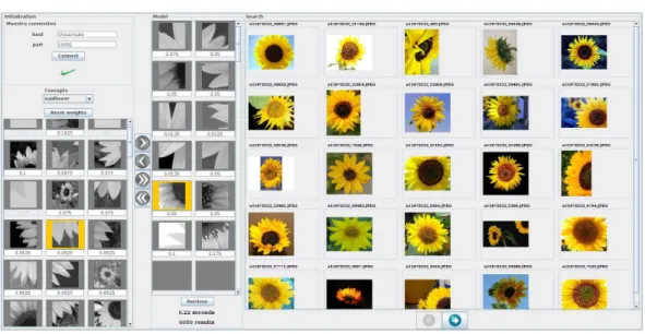
Constructing specialized visual models
Each visual patch selected as well as its weight is displayed in the middle panel representing the specialized model. The double-right arrow and the double-left arrow are used to add the entire model to the center panel and to clear it, respectively. These images are displayed in the right panel along with extra information about retrieval time and the total number of images returned.
Refining the visual model
Now, let's look at the example shown in Figure 5.4 and notice the difference between the first listed results. Unlike the previous example, the images taken here tend to occupy the entire image area. The first question focuses on the upper front part of the zebra (the head) while the second question is more of a general and global view of a zebra.

Experiments
Data preparation and test conditions
- Datasets
- Local features
- Algorithm parameters
- Evaluation metrics
Note that the number of practice images shown corresponds to the number of positive images. We kept approximately equal numbers of positive and negative images for each category of objects we trained on. However, the number of relevant images used in prediction is equal to the number used in training.

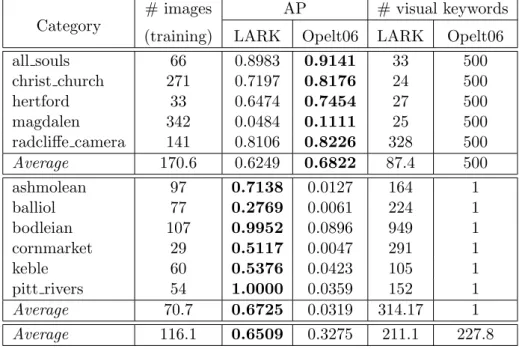
Comparison with [Opelt 2006]
- Average precision and prediction time
- Overtraining: the effect of increasing the model size
- Overfitting phenomenon
The common point between the first and the third group is that the number of features selected by LARK is less than that selected by Opelt06—which is not the case for the second and the fourth groups. Furthermore, in the three other datasets (i.e., where Opelt06 is better), we see that the average number of features in the Opelt06 model is always 500. It was only in PlantLeaves V2 that the number of features selected by LARK was greater than the number of features selected by Opelt06.

Generalization capabilities
We note that the visual keywords learned from the BeeldNetSmall training set outperformed the Caltech models in six categories and that they also outperformed on average. This proves that the models generated are generic in the sense that they do not degrade and even improve retrieval results. Performance evaluation is to gather the camel, penguin, snail and zebra categories under the concept animal, then the laptop, revolver, tennis racket and watch categories under the concept man-made and finally the sunflower and tomato categories under the concept vegetation .
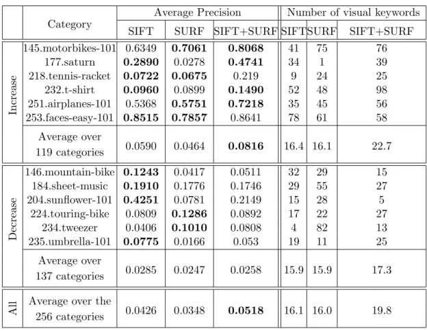
Combining multiple visual features
However, we consider these results to be satisfactory, as the increase in AP (i.e. 30%) is greater than the increase in the number of features (i.e. 26%). Additionally, keeping fewer than twenty visual keywords is appropriate from an interpretability perspective. This means that the overall performance (i.e. averaged over all object categories) of descriptor combinations is better than using one descriptor at a time and that the number of visual keywords selected by descriptor combinations is greater than the number of visual keywords selected by any single descriptor , used alone.
Adding a counter-class model
Let us take a weak classifier h′ belonging to the counterclass and suppose that it is associated with the feature F′ and the discriminative radius R′. In other words, saying that there are negative objects in the image does not necessarily mean that there are no positive objects. This behavior, although correct, creates a serious problem by neglecting the object we are looking for.

Geometric consistency
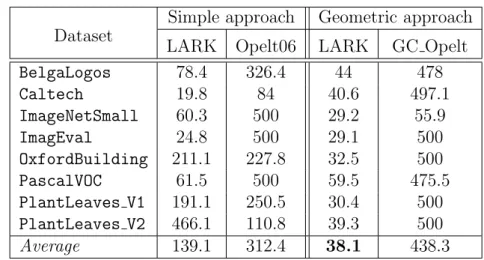
Both the BelgaLogos and OxfordBuilding datasets showed an increase in performance using the geometric approach with either LARK or GC Opelt. Looking at the forecast time (see table 6.17), we conclude that the increase of GC Opelt AP relative to LARK AP is objectively not favorable since the forecast time required for GC Opelt models is nine times (respectively almost thirteen times) longer. much longer than the time needed by LARK models to predict in BelgaLogos (respectively OxfordBuilding). On average, the prediction time from the GC Opelt models is seven times longer than the prediction time from the LARK models.
Using an efficient index structure
As expected, we observe that the performance of the exhaustive mode is always better with the simple approach (7.8% gain in AP on average). For ImagEval and with α = 0.8, notice that the AP with the geometric approach (cf. Table 6.20) is slightly larger than the AP with the simple approach (cf. Table 6.19). This was not the case for the exhaustive search, where the simple approach clearly outperformed the geometric consistency approach.
How interpretable are our visual key- words?
- Visual interpretation of the quantitative results
- Interpretability of visual keywords ambiguity
- Description limitation
- Applying geometric consistency
In this section, we provide some explanations of the experiments described in the previous chapter. We notice that among the large number of visual keywords selected by Opelt06, many are repeated. 137 allows all five sunglasses visual keywords to match two pairs of glasses.

Interaction with the visual keywords
For the two other categories, the precision at the first levels for the specialized models is always better. The complete model consists of only two visual keywords shown at the top of the figure and their corresponding precision-recall curves are given below. Comparing the precision for the first ranked results (say 5% recall), we see that the full model behaves quite well while each feature, alone, does not.

Synthesis
AdaBoost sometimes avoids overtraining, but tends to overfit, especially with a reduced number of training images. In the second case, we noticed a slight increase in the average of the total number of visual words selected by BLasso. To reduce the ambiguity of the trained visual keywords, we then introduced an alternative approach, using local geometric constraints.
Applications
However, it is essential that botanists can work on trained visual models to control which plant organs have been selected as an identification key. We believe that LARK is suitable for such supervised learning problems where end users want to control and understand exactly what the machine has learned.
Perspectives
In Proceedings of the The 3rd Canadian Conference on Computer and Robot Vision, pages 3–, Washington, DC, USA, 2006. In CIVR ’07: Proceedings of the 6th ACM international conference on Image and video retrieval, pages 33–. Proceedings of the 2006 IEEE Computer Society Conference on Computer Vision and Pattern Recognition, pages Washington, DC, USA, 2006.