Joint state and parameter estimation for distributed mechanical systems

HAL Id: hal-00175623

https://hal.archives-ouvertes.fr/hal-00175623

Submitted on 5 Jun 2013

HAL is a multi-disciplinary open access archive for the deposit and dissemination of sci- entific research documents, whether they are pub- lished or not. The documents may come from teaching and research institutions in France or abroad, or from public or private research centers.

L’archive ouverte pluridisciplinaire HAL, est destinée au dépôt et à la diffusion de documents scientifiques de niveau recherche, publiés ou non, émanant des établissements d’enseignement et de recherche français ou étrangers, des laboratoires publics ou privés.

Joint state and parameter estimation for distributed mechanical systems

Philippe Moireau, Dominique Chapelle, Patrick Le Tallec

To cite this version:

Philippe Moireau, Dominique Chapelle, Patrick Le Tallec. Joint state and parameter estimation for distributed mechanical systems. Computer Methods in Applied Mechanics and Engineering, Elsevier, 2008, 197 (6-8), pp.659-677. �10.1016/j.cma.2007.08.021�. �hal-00175623�

Joint state and parameter estimation for distributed mechanical systems

Philippe Moireau†, Dominique Chapelle†^∗, Patrick Le Tallec‡

†INRIA, B.P. 105, 78153 Le Chesnay cedex, France

‡Ecole Polytechnique, 91128 Palaiseau cedex, France

Comput. Methods Appl. Mech. Engrg.197: 659-677, 2008, doi:10.1016/j.cma.2007.08.021

Abstract

We present a novel strategy to perform estimation for a dynamical mechanical system in standard operating conditions, namely, withoutad hocexperimental testing. We adopt a sequential approach, and the joint state-parameter estimation procedure is based on a state estimator inspired from col- located feedback control. This type of state estimator is chosen due to its particular effectiveness and robustness, but the methodology proposed to adequately extend state estimation to joint state- parameter estimation is general, and – indeed – applicable with any other choice of state feedback observer. The convergence of the resulting joint estimator is mathematically established. In addi- tion, we demonstrate its effectiveness with a biomechanical test problem defined to feature the same essential characteristics as a heart model, in which we identify localized contractility and stiffness parameters using measurements of a type that is available in medical imaging.

1 Introduction

The challenges represented by estimation in distributed mechanical systems have been recently renewed and extended – in particular – by the rapidly developing applications of biomechanics in medicine [36, 4, 39]. Such problems often involve three dimensional continuum mechanics coupled to biologi- cal phenomena and they can be represented by a set of coupled partial differential equations [15, 38, 17].

But the physical parameters considered in a biomechanical model are generally very difficult to deter- minea prioriby experimentations, as living materials display very different behaviors when takenin vivo on the one hand, andpost-mortemor evenin vitroon the other hand. Moreover, for diagnosis purposes in medicine, estimation can be envisaged as a methodology to assess the condition of a patient’s living or- gan. Therefore, there is a clear interest in being able to perform estimation using available measurements of the system in “standard” operating behavior – as opposed to ad hoc experimentations – measurements that for example can be provided by medical imaging. Note that this also holds, e.g., in meteorology or more generally in geophysics. In such fields the process aiming at obtaining unknown parameters – primarily initial conditions in the dynamical systems – by using various observational data is usually referred to asdata assimilation.

As is well known, data assimilation methodologies fall into two main categories: variational and sequen- tial (or filtering) procedures. Variational procedures consist in minimizing – with respect to all unknown

∗Corresponding author:dominique.chapelle@inria.fr

parameters – a criterion based on the observation error, with the model equations taken as constraints [26, 23, 9, 22]. This leads to heavy computations in order to obtain the gradient of the criterion, generally by using the (backward in time) adjoint state, which requires extensive storage for large systems. On the other hand, sequential procedures in their classical forms – namely, Kalman filtering [21, 19, 8, 3], and related extensions to nonlinear systems – are not adapted to distributed mechanical systems because they involve the computation and manipulation – with some inversion steps – of covariance matrices that have the size of the state variable, just for estimating the state.

Regarding state estimation, however, we know from classical control and observation theory that it has close connections with control and stabilization [30]. Furthermore, since we are specifically concerned with mechanical systems, we can seek state estimators based on mechanical stabilization strategies that take into account the physical nature of the system at hand. In particular, collocated feedback is known to provide very effective stabilization strategies, both from theoretical (see [2] and references therein) and engineering perspectives [33], including with very “low-cost” (in terms of computations involved) feedback operators that can be directly used as filters in sequential state estimation.

The objective of this paper is thus to construct a joint state-parameter estimation procedure based on a simple collocated feedback strategy for state estimation, adequately extended by Kalman filtering techniques to allow the simultaneous estimation of a limited set of unknown parameters.

The outline of the paper is as follows. Section 2 describes the underlying physical models and the collocated feedback procedure which can be applied to estimate the state vector within the model. The performances of this estimation strategy is analyzed and numerically assessed in Section 3, with a de- tailed estimate of the damping properties of the proposed feedback. Section 4 introduces and analyses – both theoretically and numerically – a specific Kalman filtering technique coupled to the above feed- back procedure for the joint state-parameter estimation in a linear framework. This methodology is then extended in Section 5 to a nonlinear estimation problem where the stiffness matrix depends linearly on unknown parameters.

2 Problem statement

2.1 General framework

We consider a mechanical system in the realm of solid or structural continuum mechanics, where the acceleration field inside the body is given by the imbalance between internal stresses and external forces.

When xdenotes the state vector including displacements yand velocities ˙y, such systems are described in a linear framework by a dynamical system – underlied by partial differential equations – written in the following generic form









 dx

dt =Ax+R x(0)= x₀+ζ_x

(2.1) whereAis a linear differential operator generating a continuous semi-group, andRa source term. More specifically, this equation expresses the conservation of linear momentum, completed by the identity relating the velocity and the time derivative of displacement, namely, in a weak form,

Z

Ω

ρdy

dt ·δy dΩ = Z

Ω

ρ˙y·δy dΩ, ∀δy (2.2)

Z

Ω

ρdy˙

dt ·δy dΩ =− Z

Ω

Σy,y˙

:δe dΩ + Z

Ω

f ·δy dΩ, ∀δy (2.3)

HereΩrepresents the geometrical domain of the system,ρthe mass per unit volume,Σthe second Piola- Kirchhoffstress tensor,δyan arbitrary test function in the displacement space withδethe corresponding infinitesimal variation for the Green-Lagrange strain tensor, and fthe applied loading (taken here as a 3D distributed field to fix the ideas). Hence, in System (2.1)xdenotes the state variable y y˙T. Assuming small displacements, we can identifyδewith the symmetric part of the gradient∇δy, and takeΣ– which can then be identified with the Cauchy stress tensor – as a linear function of x. We are thus led to the linear operatorA. The differential system considered is of infinite dimension, its unknowns being the displacement and velocity fields at each point of the continuous body.

In the above system,ζx represents the unknown part in the initial conditionx(0). Likewise, we assume thatAandRdepend on a set of parameters in the form

θ=θ0+ζθ, (2.4)

in whichζθ is undetermined. Our objective is to obtain a joint estimation of the unknown quantities ζx

andζθ, based on measurements available for the system. These measurements are assumed to be given by

Z =Hx+χ

whereH is a linear operator referred to as the observation operator, andχdenotes a white noise intro- duced by the measurement procedure (detection, sampling...) that we describe in more details below. We also introduce

Z¯ =Hx (2.5)

to represent an “exact measurement” which of course is never available in practice. More specifically, in the whole paper the measurements considered will be the velocities taken in a subpartΩ_mof the domain Ω, and sampled in space by using weight functions (s_i)^q_i=1 defined onqnon-overlapping “measurement cells” withinΩ_m. Namely,Hx=(0H^v)(yy)˙ ^T consists of theqthree-dimensional vectors given by

Z

Ω_m

siy dΩ,˙

and we assume that the sampling functions are normalized, i.e.ks_ik_L2(Ωm) =1. We also assume that each of these measured vectors areindependentlyperturbed with a white noise of associated covariance matrix α²_iI3, which all together make up the above white noiseχ. Therefore, the covariance matrix ofχcan also be decomposed in the following manner:

Qχ=

q

X

i=1

(α_i)²

V_i¹(V_i¹)^T+V_i²(V_i²)^T +V_i³(V_i³)^T, (2.6) where V_i^j denotes the column vector with a 1 in the entry corresponding to the j-th coordinate (for

j=1,2,3) of thei-th cell and 0 elsewhere.

Our estimation strategy will be based on observer theory and feedback control.

2.2 Modelling and discretization

Our observer approach relies on a discretized version of the above reference model. Namely, we approx- imate x by xh where xh can be represented by a finite dimensional state vector X of dimension n. The

corresponding finite dimensional system can be written in the following formalism:











X˙ =AX+R

X(0)= X0+ζ_X (2.7)

where the initial condition expresses that x_h(0) is the interpolation (or projection) of x(0) in the finite dimensional subspace of the state space. We also introduce the operator ℑ_h as the one-to-one mapping fromRⁿ to this subspace, namely, so that xh = ℑ_hX. Like the continuous formulation, this dynamical system represents the state space form of a variational – here discrete – formulation, typically derived from (2.2)-(2.3) by using a finite element discretization. Denoting byYthe vector of degrees of freedom corresponding to the discrete displacement field, in the linear case the variational formulation yields a matrix equation of the type

MY¨ +CY˙+KY =F, (2.8)

whereM,Cand Krespectively denote the mass, damping and stiffness matrices, and Fthe load vector (see [7, 18]). WithX= Y Y˙T, we thus have the following expressions forAandRin (2.7):

A= 0 I

−M⁻¹K −M⁻¹C

!

, R= 0

M⁻¹F

!

. (2.9)

As a natural norm in the state space, we will use the energy norm, where the energy considered is the sum of kinetic energy and strain energy, namely,

kXk²_E = 1

2Y˙^TMY˙ +1

2Y^TKY, (2.10)

and we define

N = 1 2

K 0

0 M

! ,

so that kXk²_E = X^TNX. Of course, the energy norm can also be considered for the continuous state, although not with the above matrix expressions.

As regards the observation, we have

Z=HX+ǫ_h+χ, (2.11)

with

H=H ℑ_h,

ǫ_h =H(x−x_h). (2.12)

The quantityǫ_h denotes a “small” approximation error produced by the discretization procedure in the observations.

Noting thatHonly acts on velocities – like the continuous observation operatorH – we will also use the expression

H=(0 H^v).

From a practical point of view, H^v consists of the collection of consistent force vectors S_i^j, (1 ≤ i ≤ q,1≤ j≤3), associated with the loading corresponding to a distributed forces_ialong the j-th cartesian coordinate, each of these vectors being stored in a separate line ofH^v.

2.3 Model problem

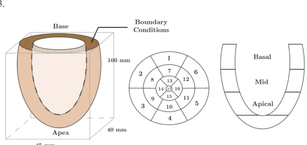
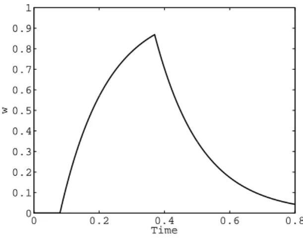
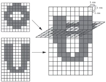
In order to illustrate and assess our estimation procedures, we will consider an example problem inspired from biomechanics and representing a simplified cardiac ventricle. The geometry of our example problem is depicted in Figure 1, and the characteristic dimensions of this object are – indeed – comparable to those of a human left ventricle. We thus resort to cardiac terminology to refer to the two extremities of the object, namely “apex and base” (see Figure). The system is clamped over the planar surface at the base, and activated by a planar wave of prestress – representing electrical activation – traveling from apex to base at wave speedc= 0.5 m.s⁻¹, which means that it takes 0.2 s for the wave to reach the base. The wave shape itself is shown in Figure 2. The resulting prestress state is assumed to be isotropic and gives an external virtual work defined by

δW^PS = X

1≤i≤17

Z

Ω^AHA

i

θiσ0w(x3−ct) Tr(δ∇y)dΩ =δY^T ·R, (2.13) where the subdivision of the solid domain into 17 sub-regions is similar to the subdivision of the left ventricle advocated by the American Heart Association, see [1]. In the case of our simplified geometry this subdivision is depicted in Fig. 1. In the above expressionσ₀denotes a constant contractility parame- ter, andθi a multiplicative coefficient that may take a different value in the range [0,1] within each AHA region to represent pathological contraction. Namely, settingθ_i < 1 in a given region corresponds to a simplified model of infarcted tissue in that area, hence the parameters (θ_i)1≤i≤17 represent the quantities to be estimated for diagnosis purposes. In our reference simulations we take all these parameters to be 1 (healthy value) except for

θ₁₄ =0.5, (2.14)

see Figure 3.

1 6

5 4 3

2 ⁷

12

11 10 8

9 13 14

15 16 17

Apical Mid Basal

Apex

Base Boundary

Conditions

45 mm

40 mm 100 mm

Figure 1: Model geometry (left) and AHA regions (center and right)

Our simulations will correspond to an isotropic viscoelastic material in linear analysis, with material parameters given by

Ei =12.6 10³Pa, νi=0.3, ηi =0.227 s ∀i∈ {1, . . . ,17}, (2.15) and respectively denoting Young’s modulus, the Poisson ratio and a viscoelastic coefficient associated with the pseudo-potential

W^v =η_i λ_i

2(Tr ˙ε)²+µ_iTr(˙ε²)

, ∀i∈ {1, . . . ,17},

0 0.2 0.4 0.6 0.8 0

0.1 0.2 0.3 0.4 0.5 0.6 0.7 0.8 0.9 1

Time

w

Figure 2: Activation profilew

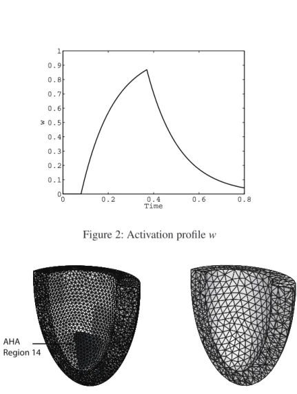
AHA Region 14

Figure 3: Reference mesh with ‘infarcted’ region (left) - ‘Desired’ mesh to be used in estimation (right)

whereλ_ietµ_iare the Lam´e constants derived fromE_i andν_i, and ε= 1

2 ∇y^T+∇y

denotes the linearized strain tensor approximating – at the first order – the Green-Lagrange deformation tensor in the small displacements framework. Note that this viscoelastic contribution corresponds to stiffness-based Rayleigh proportional damping. This leads to the following constitutive law to be taken into account in the variational formulation

Σ =λiTr(ε+ηiε)1˙ +2µi(ε+ηiε).˙ (2.16) Also, volumic mass is set asρ=10³kg·m⁻³,a standard value for biological tissues.

The measurements used in the estimation procedures will be provided by a “reference model” given by a rather fine finite element discretization of the above object. The corresponding mesh is displayed in Figure 3 and features nearly 40000 degrees of freedom. The observer itself will be based on coarser discretizations, where the adequate mesh size will be a matter of discussion in the sequel. In all our simulations we used for time discretization the energy-conserving Newmark algorithm with time step

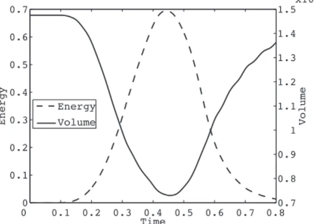
∆t=1 ms. This time step is adequate for accurately representing the first 1000 eigenmodes of the system with at least 20 time steps per modal period, but is primarily determined in relation to the activation wave velocity. We show in Figure 4 the resulting energy and internal volume profiles for the reference simulations. Note that – unless otherwise stated – all physical units correspond to the SI system. We point out that internal volume is an important medical indicator and that our numerical values are “realistic”

in this respect.

0 0 0.1 0.2 0.3 0.4 0.5 0.6 0.7 0.8 0.1

0.2 0.3 0.4 0.5 0.6 0.7

Time

Energy

Energy

0.7 0.8 0.9 1 1.1 1.2 1.3 1.4 1.5x10⁻⁴

Volume

Volume

Figure 4: Energy and volume of the cavity for the reference solution

Finally, the measurement cells introduced above are defined by subdividing a (rectangular) box enclos- ing the geometry into 10×10×15 smaller (rectangular) cells of equal sizes. This subdivision is visualized in Figure 5. The weight functions are then simply defined by scaled indicator functions of the cells. We point out that this resolution is comparable to that of standard tagged MRI images.

1 cm 1 cm 1 cm

Figure 5: Measurement cells

2.4 State estimation using collocated damping

We now introduce the finite dimensional state estimator of our original system (2.1)











X˙¯ =AX¯ +R+K_X(Z−HX)¯ X(0)¯ = X0

(2.17) This state estimator uses the unbiased estimate of the initial condition and corrects the dynamics of the discrete system by a feedback proportional to the measured error. In essence, the filterKXthat we want to use corresponds to a force proportional and opposed to the measured velocity, namely a “direct velocity feedback” (DVF) stabilization strategy, see [33, 10]. This is the simplest type ofcollocated feedback, namely a feedback law in which the control applied in a given location only uses the measurement corresponding to that location. In our case, the available measurements are weighted velocities within cells, hence inside each cell we want to apply a “filtering force” given by

−γs_i Z

Ω_m

s_iy dΩ.˙

Noting that the corresponding variational form of this feedback reads

−γ Z

Ωm

s_iy dΩ˙ Z

Ωm

s_iδy dΩ,

we infer thatKX is simply given by

KX =(0 γH^vM⁻¹)^T.

Hence, the dynamics of the associated mechanical system is governed by

MY¨¯ + C+γ(H^v)^TH^vY˙¯ +KY¯ = F+γ(H^v)^TZ, (2.18) where the dissipative effect of the filter clearly appears through the positive factorγ(H^v)^TH^v. Note that this matrix is straightforward to compute in a mechanical finite element software, and that collocation induces a very narrow bandwidth, whereas Kalman filtering would yield full matrices.

3 Analysis of the state estimator

We point out that – in our mathematical error estimates – we use the symbolC to denote a generic positive constant that may take different values for all occurrences.

3.1 General framework

Let us define the error ˇXbetween (2.7) et (2.17), namely, Xˇ = X−X,¯ whose dynamics is given by











X˙ˇ =(A−K_XH) ˇX−K_X(ǫ_h+χ) X(0)ˇ =ζX

(3.1)

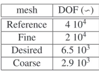
mesh DOF (∽) Reference 4 10⁴

Fine 2 10⁴ Desired 6.5 10³

Coarse 2.9 10³

Table 1: Number of dofs for the computational meshes

A straightforward computation shows that the covariance matrix of the vectorKXχis of ordern– with n very large in finite element applications – and given by

Q=









0 0

0 γ²Pq i=1

P₃

j=1(α_i)²M⁻¹S_i^j(S_i^j)^TM⁻¹







. (3.2)

Considering (3.1), in order to drive the above estimation error to zero, we are concerned with the properties – and more particularly the stability – of the dynamical system governed byA−K_XH, namely, the discretized form of a mechanical system with dissipative feedback. It is known that, under certain assumptions regarding the location and extent ofΩ_m, in the infinite dimensional case this closed-loop system is asymptotically exponentially stable in the energy norm, see in particular [27, 6]. However, such theoretical results do not provide quantitative estimations of exponential stability constants, which we are much concerned with. In addition, in our case the observer is based on a discrete system for which stability properties must be specifically investigated. We thus undertake this investigation by analysing the poles of the system considered, namely the eigenvalues of (A − KXH). As is well established in control theory (see [13] and references therein), this allows quantitative estimation of stability properties.

Nevertheless, in our case a particular attention is necessary as to how these properties may be affected when changing the space discretization, since this constitutes a “modeling parameter” that may be varied in the observer formulation, in particular in order to improve the accuracy. Hence, we now present a numerical study of the poles for the above example problem with various values ofγand several choices of discretizations.

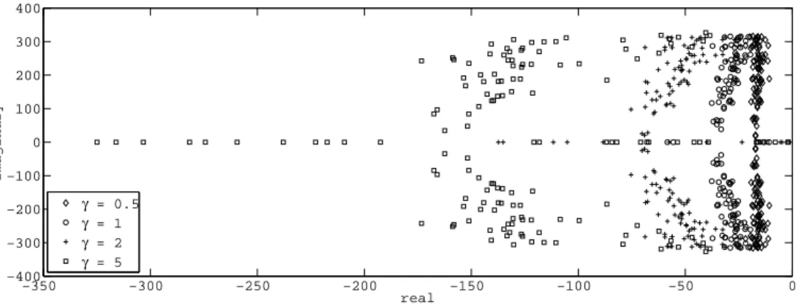
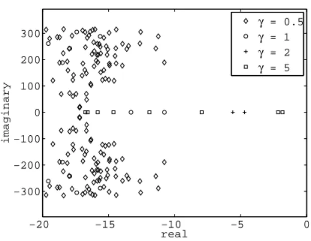
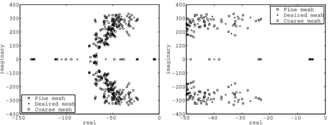
We show in Figure 6 the root locus of the first 150 eigenmodes for four different values of the gain parameterγ, with a zoom near the imaginary axis in Fig. 7. These eigenpairs are computed with a mesh corresponding to about 6500 degrees of freedom – henceforth referred to as the “desired mesh” – but we show in Figure 8 that the dependence of the stabilization effect on the discretization is of no serious concern, see Table 1 for the sizes of the meshes considered. We point out that the “desired mesh” was deliberately selected with a limited number of degrees of freedom in order to provide fast computations in the estimation procedure, while representing a “reasonable” discretization of the geometry, see Figure 3. Of course, we will be concerned with the errors induced by this discretization, much coarser than that used in the reference simulations, and we will assess these discretization errors in our forthcoming analyses.

3.2 Damping properties of the collocated system

Although the above numerical results indicate a very effective stabilizing effect for our collocated feed- back, these results only concern – of course – a limited number of poles, and – furthermore – provide no information on the associated eigenvectors, in particular as to how well they “span” the state space.

Therefore, they only give an incomplete description of the dynamics of the error system (2.18). For a

−350 −300 −250 −200 −150 −100 −50 0

−400

−300

−200

−100 0 100 200 300 400

real

imaginary

γ = 0.5 γ = 1 γ = 2 γ = 5

Figure 6: Root locus for different values ofγ(units in s⁻¹)

−20 −15 −10 −5 0

−300

−200

−100 0 100 200 300

real

imaginary

γ = 0.5 γ = 1 γ = 2 γ = 5

Figure 7: Zoom on the root locus near imaginary axis

−150 −100 −50 0

−400

−300

−200

−100 0 100 200 300 400

real

imaginary

Fine mesh Desired mesh Coarse mesh

−50 −40 −30 −20 −10 0

−400

−300

−200

−100 0 100 200 300 400

real

imaginary

Fine mesh Desired mesh Coarse mesh

Figure 8: Stability of the root locus w.r.t. mesh discretization (near imaginary axis)

continuous system, a desirable related feature is that the eigenvectors make up a Riesz base [13, 37].

This can be mathematically established for the corresponding one-dimensional problem, see [12]. How- ever, there is no such general result in 2D or 3D or in elasticity, in particular due to geometrical effects [24, 25]. Nevertheless, for practical purposes it is not necessary to take into account the full complex- ity of the spectral problem – and in particular as regards the behavior of the numerical and physical high frequencies and modes – in order to evaluate the rate of exponential stability for the sequence of homogeneous dynamical systems











X˙ˇhg=(A−KXH) ˇXhg

Xˇ_hg(0)=ζ_X (3.3)

Indeed, a “real” initial conditionx(0)= x0+ζxis in general sufficiently regular to be well approximated by only “a few” eigenmodes of the system without stabilizer. The discrete solution at any time can then be bounded using the following result, where we denote by (Φ_i, λ_i) and (Ψ_i, µ_i) the complex eigenpairs ofAandA−KXH, respectively – assuming that these eigenpairs are arranged in ascending order of the associated eigenfrequencies.

Proposition3.1

Assume that for System (3.3) the initial condition can be expanded in the modal basis{Φ_i}of the original system as

Xˇhg(0)=

q

X

i=1

αiΦ_i+rq.

Then, for any timetwe have the bound kXˇhg(t)k_E ≤C(q^′)e^−δ(q′)t 1+d(q,q^′)

kXˇhg(0)k_E+kr_qk_E

+kr_qk_E+d(q,q^′)

kXˇhg(0)k_E+kr_qk_E , (3.4) where the constants appearing in this estimate are defined as follows,

δ(q^′)= inf

i≤q^′ −ℜ(µ_i) ,

d(q,q^′)= sup

V∈span(Φ_i)^q_i=1

inf

W∈span(Ψ_i)^q_i=1^′

kV−Wk_E kVkE

,

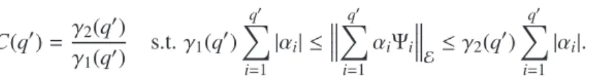
C(q^′)= γ₂(q^′)

γ1(q^′) s.t. γ₁(q^′)

q^′

X

i=1

|α_i| ≤

q^′

X

i=1

α_iΨ_i

_E ≤γ₂(q^′)

q^′

X

i=1

|α_i|.

The estimate (3.4) is straightforward to establish, and it means that, once the initial condition is decom- posed using the modes of the original system (up to some “small” remainderr_q), the state at all times can be bounded using the poles of the collocated system withℜ(µ_i) the real parts of the corresponding eigenfrequencies. The constant d(q,q^′) represents the distance between the subspaces spanned by the eigenvectors{Φ_i}and{Ψ_i}of the original and collocated systems, andC(q^′) the constant of equivalence of norms between the energy norm and the norm associated with modal components. It can be checked numerically (by computing the corresponding Rayleigh quotients) that d(q,q^′) is “small” as soon as q^′ ≥ q, and thatC(q^′) remains finite, both properties being obtained rather independently of the mesh considered. This can be seen as a numerical verification of the fact that the collocated eigenvectors ad- equately span the state space – the numerical counterpart of the above-mentioned Riesz basis property, valid at least for the low frequencies which are the main concern in our case.

Hence we are led to an estimate of the type

kXˇ_hg(t)k_E ≤C₁e^−δ1tkXˇ_hg(0)k_E+ε, (3.5) whereδ1 is related to the poles positions of the collocated system, andεdenotes a small quantity. Our aim is thatδ₁ .T >>1, which expresses that the exponential stability is meaningful with respect to the time constant of the dynamics. In other words, we want to estimate quantitatively the time constant of the stability, and analysing the poles is a way to achieve such an estimation whereas abstract results on exponential stability usually just provide the existence of such an exponential estimate. In this respect, only limited semi-quantitative results are available – see e.g. [33] – such as the following expression for the sensitivity of the poles position with respect toγ

dµ_i

dγ(0)= dℜ(µ_i)

dγ (0)=−W_iH^THW_i 2

whereWidenotes thei-th mass-normalized displacement eigenvector of the original system, namely such that

KW_i=λ_iMW_i, W_i^TMW_i=1.

We now illustrate this discussion with some numerical simulations obtained with our example problem.

Figure 9 displays the effect of an error in the initial condition corresponding to a static displacement obtained by imposing an internal pressure of 10³ Pa, which is the order of magnitude of the pressure induced by atrium contraction during ventricular filling. The quantity shown is the energy (in base 10 log) of the simulated state corresponding to System (3.3). We can distinguish two parts in the resulting evolutions, corresponding to two clearly distinct stabilization rates for each choice ofγ. The first slope is related to the eigenmodes which dominate in the initial condition, while the second one corresponds to the least stable poles that are led to the real axis due to the damping added by the collocated stabilizer, recall Figs. 6–7. Note that the asymptotic behavior may also be conditioned by some high frequencies – whether they be physical or purely numerical as discussed in [5] – which is not observed here. We can see in Figure 9 that the choiceγ = 2 is optimal as regards the initial slope, and that the corresponding asymptotic slope is associated with errors that are of no practical concern.

Unless otherwise indicated, we will use the static displacement produced by the above internal pressure as the initial state error in our numerical estimation experiments in the sequel.

0 0.2 0.4 0.6 0.8 10⁻¹⁵

10⁻¹⁰ 10⁻⁵ 10⁰

Time

Error

γ = 0.5 γ = 1 γ = 2 γ = 5

Figure 9: Energy for initial condition error (log scale)

3.3 Influence of measurement and discretization errors

Let us now concentrate on the influence of the right-hand side KX(ǫh + χ). In this matter, we distin- guish between the deterministic termK_Xǫ_hand the probabilistic oneK_Xχ. The main difference with our previous analysis is that we cannot assume any space regularity on these terms and they may – indeed – include some high frequency contents. As a consequence, we will consider both the case of uniformly exponential stability and the case where we only have stability in the error system (3.1). To that end we define – independently of the discretization in all cases – two positive constantsδandCsuch that:











δ .T >>1 if uniformly exponential stability

δ=0 if only stability (3.6)

This allows to bound the (discrete) semi-groupT^h(t) generated by the operator (A−KXH) as

kT^h(t)k ≤Ce^−δt, (3.7)

which in turn will provide bounds on the errors.

We first consider the effect of the probabilistic termK_Xχ. To that purpose we can analyze the dynamical system











X˙ˇχ=(A−KXH) ˇXχ−KXχ

Xˇ_χ(0)=0 (3.8)

The random variable ˇX_χis then Gaussian, hence characterized by the behavior of its mean and covariance.

We obviously haveE( ˇX_χ)= 0 for the mean. In order to deal with the covariance we use the semi-group formulation and obtain

E(kXˇχk²_E)= Z T

0

Tr Q(T^h(t−τ))^TNT^h(t−τ) dτ

where Q is the covariance of the white noise KXχ and N is the energy norm matrix. Substituting the expression in (3.2) and using (3.7), we directly obtain

E(kXˇ_χk²_E)≤C₂T₂γ²

q

X

i=1

α²_i, (3.9)

with

T2=











1/δ≪T if uniformly exponential stability

T if only stability (3.10)

The influence of observation noise is illustrated with our example problem. We took a white noise standard deviation corresponding to ten percent of a reference velocity value in our simulations for a sampling rate of 50 ms. When rescaled according to white noise rules to the actualcomputationaltime step, this corresponds to a standard deviation of about 70 percent of the reference value. We show in Figure 10 the energy of the solution ˇX obtained with various values of the observer gainγ. As expected

0 0.2 0.4 0.6 0.8

10⁻⁸ 10⁻⁷ 10⁻⁶ 10⁻⁵ 10⁻⁴

Time

Error

γ = 0.5 γ = 1 γ = 2 γ = 5

Figure 10: Error induced by measurement noise (energy in log scale)

from the above numerical analysis, the gain has an amplification effect on the noise which is of the type predicted by (3.9). Nevertheless, we can see that for all values ofγof interest, the error associated with the noise is rather small – and indeed not dominant compared to the modeling error that we will now investigate.

We thus complete our stability analysis with the study of the the deterministic source term K_Xǫ_h. Namely, we consider the system











X˙ˇ_d =(A−K_XH) ˇX_d−K_Xǫ_h

Xˇ0 =0 (3.11)

Using Duhamel’s formula we obtain Xˇ_d(t)=

Z _t

0

T^h(t−τ)K_Xǫ_h(τ)dτ and we infer the following estimation for the deterministic right-hand side

kXˇd(t)kE≤Cγp

T2kx−xhk_L2([0,T];E). (3.12)

We can summarize the convergence of our state estimator in the following estimate combining the contributions of initial error, discretisation error, measurement noise, and high frequency cut-off.

E(kXkˇ ²_E)≤Ch

e^−2δ1tE(kζ_Xk²_E)+T2γ²kx−xhk²_L2([0,T];E)+T2γ²

q

X

i=1

α²_i +ε²i

. (3.13)

We give the corresponding numerical results in Figure 11, where we clearly see that the modeling error – here due to the discretization – is dominant in the error after the initial condition error has been damped according to the above discussion. As expected this modeling error only arises with the occurrence of the activation wave. We also remark that the modeling error effect is quite stable in the range ofγ chosen, and that we do not observe the amplification effect ofγthat could be expected from (3.13).

0 0.2 0.4 0.6 0.8

10⁻⁵ 10⁻⁴ 10⁻³ 10⁻² 10⁻¹

Time

Error

γ = 0.5 γ = 1 γ = 2 γ = 5

Figure 11: Global error with respect toγ(energy in log scale)

Eventually, in order to assess the dependence of our procedure with respect to the discretization, we give in Figure 12 the results obtained with observers based on three different meshes – recall Table 1 – with measurements generated from the same above-defined reference mesh. We conclude that the effect of the discretization is roughly as predicted from (3.13). Also, we compare in Figure 13 the estimation error for the desired mesh with the errors associated with

• the solution of the direct problem (2.7) generated with the desired mesh without initial condition error (this gives the curve labeled “discretization error” in Fig.13);

• the reference solution interpolated in the desired mesh at each time step (the “interpolation error”).

This comparison shows that – after a short time corresponding to the stabilization of the collocated system – the observer provides an estimation withoptimal accuracyas compared with the interpolation error. The estimated state is indeed superior to the solution directly simulated on the desired mesh for the period of maximum energy, despite the very small time step that reduces – in the direct solution – the error due to the approximation of high frequency dynamics. This – of course – is only possible because of the feedback provided by the measurements in the observer.

4 Joint state-parameter estimation: the linear case

4.1 General framework

In this section, we consider the estimation of parameters only included in the right-hand side of the dynamical equation, and with alineardependence on the parameter vectorθof dimensionr. Hence, we

0.1 0.2 0.3 0.4 0.5 0.6 0.7 10⁻⁶

10⁻⁵ 10⁻⁴ 10⁻³ 10⁻² 10⁻¹

Time

Energy

Fine mesh Desired mesh Coarse mesh Solution

Figure 12: Global error with respect to the discretization (energy in log scale andγ=2)

0 0.2 0.4 0.6 0.8

10⁻⁸ 10⁻⁶ 10⁻⁴ 10⁻² 10⁰

Time

Error

Discretization error Interpolation error State estimation error System Energy

Figure 13: Comparison of estimation, interpolation and discretization errors can write the following linear state-parameter system:















˙

x=Ax+Bθ+R x(0)= x₀+ζ_x θ=θ0+ζθ

(4.1)

whereζ_θrepresents the unknown part in the parameters.

If the parameters were perfectly known we could apply the above state estimation procedure. Therefore, we have formally

∀ζ_θ, lim

t→∞kx¯_h(t, ζ_θ)−x(t, ζ_θ)k=O(h^p)+noise. (4.2) But since we do not knowζ_θ the state-estimator ¯X (and equivalently ¯x_h) is unusable as such. Our main objective here is to propose an estimator ˆXwhich can start fromθ₀– notθ₀+ζ_θ– and estimate the pair

(ζ_X, ζ_θ). This is what we call joint state-parameter estimation, also referred to as adaptative observation in [41, 42].

4.2 Construction and analysis of the estimation procedure

Since we want to jointly estimate the state and the parameters, we could think of using filtering proce- dures – such as Kalman filtering – on the (discrete) system describing the evolution of the “augmented state” incorporating the parameters with the actual state (as described in [11]), namely,











X˙^e =A^eX^e+R^e

X^e(0)=X^e₀+ζ^e (4.3)

where

X^e = X θ

!

, A^e= A B

0 0

!

, R^e = R 0

!

, (4.4)

and

X₀^e = X0

θ

!

, ζ^e= ζX

ζ_θ

!

. (4.5)

However, the size of the augmented state vectorX^e, namely, 2n+r, makes classical filtering techniques – which would also not take advantage of the state estimator introduced above – untractable for this problem. Thus, we aim at building a joint state-parameter estimator based on the “cheap” state estimator X. Therefore we define the system describing the dynamics of ¯¯ X^e=( ¯X θ)^T, viz.











X˙¯^e=A^eX¯^e+R^e+K^e_X(Z−H^eX¯^e)

X¯^e(0)=X₀^e+ζ_θ^e (4.6)

where

ζ_θ^e = 0 ζθ

!

, K^e_X = K_X 0

!

, H^e =(H 0).

Here we point out that ¯X^e only depends on the initial conditionζθ. Hence we can define ¯X^e[ξ] for an arbitrary initial conditionθ(0)=θ₀+ξ.

Our idea is to apply a Kalman filtering procedure on System (4.6). Two difficulties are to be noted in this respect: (1)Zis not the observation corresponding to ¯X^ebut tox; (2)Z, which contains some (unknown) noise, is in the right-hand side of the system observed, hence this introduces some modeling noise in the state equation. In order to circumvent these difficulties in a first stage, we introduce the additional auxiliary system











X˙¯_a^e=A^eX¯_a^e+R^e+K^e_X( ¯Z−H^eX¯^e_a)

X¯_a^e(0)=X₀^e+ζ_θ^e (4.7)

using the abstract observation without noise defined in (2.5). Considering also the “virtual” observation

Z_a= HX¯^e_a+χ, (4.8)

we define ˆX_a^e as the Kalman observer for this system (4.7) when using the virtual observation Za. The error covariance of this observer, namely,

P^e_a=E(( ¯X_a^e−Xˆ_a^e)( ¯X_a^e−Xˆ_a^e)^T|Z_a) (4.9)

is such that

P^e_a(0)= 0 0 0 E(ζθζ_θ^T)

!

. (4.10)

Therefore, we are then in a position to apply Kalman filtering to a system with reduced rank covariance error. As shown in [32], in the absence of model noise, the covariance matrix at every time remains of constant rankr, namely, the size of the parameter vector. This leads to the so-called “Singular Evolutive Extended Kalman” (SEEK) algorithm in which the evolution equation ofP^e_ais:



























P^e_a=L^eU⁻¹L^eT L˙^e =(A^e−K^e_XH)L^e L^e(0)=(0 I_r)^T U˙ =L^eTH^eTW⁻¹H^eL^e U(0)= E(ζθ.ζ_θ^T)−1

(4.11)

whereW denotes the covariance matrix of the observation noise χ. If we decompose the equation de- scribingL^easL^e=(LX Lθ)^T we have in our case























L˙_X =(A−K_XH)L_X +BL_θ L˙θ =0

L_X(0)=0 L_θ(0)=I_r

(4.12)

HenceLθ =Ir,∀t, which implies

L˙_X =(A−K_XH)L_X+B, (4.13)

and

U˙ =L^T_XH^TW⁻¹HL_X. (4.14)

Finally, Kalman filtering specialized for the auxiliary system (4.7) gives the following observer equations























X˙ˆ_a= AXˆ_a+Bθˆ_a+R+K_X( ¯Z−HXˆ_a)+L_Xθ˙ˆ_a θ˙ˆa=U⁻¹L^T_XH^TW⁻¹(Za−HXˆa)

X(0)ˆ =X₀ θ(0)ˆ =θ0

(4.15)

withL_X and Urespectively given by (4.13) and (4.14), and we note that we only need to manipulate a matrix of sizer (namely, U), instead of a covariance matrix with the size of the extended state, which makes the computation of the filter tractable. We emphasize that this rank reduction was achieved by considering the (stabilized) state estimator instead of the original state equations in the augmented system (4.7), which in essence amounts to “canceling” the uncertainty associated with the state initial conditions.

This differs from the SEEK approachper se, in which rank reduction is performed by retaining only the dominating singular values in the global covariance matrix. Here, the uncertainty considered has the same dimension as the complete parameter space.

Of course, the observer ˆXacannot be used as such, since neither ¯Z norZaare available. We then resort to the natural idea of substituting the actual measurementsZfor these two quantities, which provides the

following system.















































X˙ˆ =AXˆ +Bθˆ+R+K_X(Z−HX)ˆ +L_Xθ˙ˆ θ˙ˆ =U⁻¹L^T_XH^TW⁻¹(Z−HX)ˆ

L˙X =(A−KXH)LX+B U˙ = L^T_XH^TW⁻¹HL_X X(0)ˆ =X0

θ(0)ˆ =θ0

L_X(0)=0

U(0)= E(ζθ.ζ_θ^T)−1

(4.16)

Note that Z differs from ¯Z only by the noise, and thatZa converges to a numerical approximation of Z with the time constant of the collocated closed-loop system, see Section 2. Through this substitution we lose the “theoretical optimality” associated with Kalman filtering in the reduced covariance rank framework (namely, SEEK). However, we can still establish an optimality result in a variational context.

Theorem4.1

Considering the variational criterion JT(ξ)= 1

2ξ^TU(0)ξ+ 1 2

Z T

0

(Z−H^eX¯^e(ξ))^TW⁻¹(Z−H^eX¯^e(ξ))dt, (4.17) there exists a unique minimizer ˆξand the system (4.16) is such that

X(Tˆ )=X¯^e[ ˆξ](T), ∀T ≥0. (4.18)

⋄Proof:

In order to obtain the minimizer, we differentiateJ_T dJ_T(ξ).h=ξ^TU(0)h−

Z _T

0

(Z−H^eX¯^e)^TW⁻¹H^edX¯^e dξ .h dt where











d dt

dX¯^e

dξ =(A^e−K_X^eH^e)^d_dξ^X¯e

dX¯^e

dξ (0)=(0 I_r)^T Let us introduce the adjoint variable p^esatisfying











p˙^e+(A^e−K^e_XH^e)^Tp^e= H^eTW⁻¹(Z−H^eX¯^e) p^e(T)=0

Then,

dJT(ξ).h = ξ^TU(0)h− Z T

0

( ˙p^e+(A^e−K_X^eH^e)^Tp^e)^TdX¯^e dξ .h dt

= ξ^TU(0)h+ Z T

0

p^eT d

dt dX¯^e

dξ −(A^e−K^e_XH^e)dX¯^e dξ

.h dt

−

"

p^eTdX¯^e dξ .h

#T

0

= (0 Ir)p^e(0)+U(0)ξT.h