Knot invariants in embedded contact homology

Une structure de contact sur Y est une distribution de faces ξ pour laquelle il existe une forme de contact α avec ξ = kerα. Suite à ce théorème, il est naturel de chercher un analogue dans l'homologie de contact encastrée de l'homologie de Heegaard Floer pour les nœuds.

Holomorphic curves

If δ is Reeb's orbit associated with the puncturex, then a pair of x determines a cover of δ: the number of sheets of this cover is the local x-multiplicity of δ in u. The sum of the x multiplicities over all punctures x associated with δ is the (total) multiplicity of δ inu.

Morse-Bott theory

A Reeb-expanded torus T circling all in the same class H1(T) (such as the Morse-Bott torus) can be used to obtain constraints on the behavior of a holomorphic curve near T. Let T be a linear Reeb-expanded trajectory with slope s=s(T) and u holomorphic curve are as above.

Open books

In section 2.3 we recall the definition of the periodic Floer homology groups for open books. Finally, in section 2.4 we recall the definition of the version of ECH\ for homologically trivial nodes.

ECH for manifolds with torus boundary

ECH and ECH d from open books

Periodic Floer homology for open books

Another Floer homology theory closely related to ECH is the periodic Floer homology denoted P F H and defined by Hutchings (see [26]). Then P F H(N(S, φ)) is defined in a similar way to ECH for an open book, but by replacing the Reeb vector field with a stable Hamiltonian vector field R parallel to ∂t where the coordinate is [0,2] : we refer the reader on [26]. If α is a contact form adapted to (S, φ), then there exists a stable Hamiltonian structure such that for every i≥0,.

ECH d for knots

This is indeed the actual ECH difference of the manifold Y \int(V(K))(and not the restriction of the ECH difference of Y to the orbital sets in Y \int(V(K))). Due to the abundance of literature on the argument, we will show only some aspects of the construction. Finally, in section 3.3 we recall the interpretation of the multivariable Alexander polynomial∆L of a link L⊂S3 in terms of the dynamics of suitable vector fields in S3\L.

All Heegaard Floer homology groups of Y do not depend on any of the choices made and are topological invariants of Y. This is a kind of double Poincare version of the fact that ∂ECH obeys the first homology of generators of the chain ECH groups .

Heegaard Floer homology for knots and links

The knot ltration

Now let ∂HF K be the part of ∂HF that preserves the ltration given by equation 3.2.4, which in this case is the map restricting the count of ∂HF to the holomorphic curves u with nz(u) = nw (u ) = 0. A further version of HFC is obtained by taking the homology of the subcomplex CF K−(Σ,α,β, w, z)or CF K∞(Σ,α,β, w, z) freely generated by the triples[x, i, j] with i < 0. Endowed with the constraint of the differential, this gives the minus version of Heegaard Floer knot homology of K HF K− (K, Y).

By arguments similar to the case of knots, equation 3.2.6 induces a Zn ltration on suitable Heegaard-Floer complexesCF−(S3) and CFd(S3)denet using special Heegaard diagrams for S3 compatible with L. The first sides of the spectral sequences in the two versions the Heegaard-Floer link homologies are HF L−(L, S3) and HF L(L, S[ 3).

HFL and Alexander polynomial

Now these homology groups inherit (from Eq. 3.2.6) a gradation of Zn or, analogously, n degrees of Z, one for each component of L. The quotient means that the Alexander polynomial is well defined only up to multiplication by monomials of the form ±ta11· · ·tann . The fact that the Alexander polynomial is defined up to the multiplication of terms of the form ±ta11· · ·tann depends on the choice of raising the basis H1(S3\L) to the basis for the homology of the universal abelian cover from S3 \L.

An equivalent ambiguity also occurs in HF L and HF K when choosing to raise relative degrees to absolute degrees. In the next section, we will recall the definition of ∆L in terms of the dynamics of certain vector fields defined in the complement of the link.

A dynamical formulation of ∆(t)

Twisted Lefschetz zeta function of ows

With these data it is possible to define the Lefschetz sign of γ, exactly as we did in Section 1.1 for orbits of Reeb vector fields associated with a contact structure ξ, but now with TxD instead of ξx. Indeed, it is possible to prove that the Lefschetz sign of γ does not depend on the choice of x and D and that it is an invariant (γ)∈ {−1,1} of φR near γ. When ρ is understood, we write ζ(φR) directly and call it the twisted Lefschetz zeta function of φR.

We note that in [16] the author denesζρ(φR) in a slightly different way and then he proves (Theorem 2) that, under some assumptions that we will state in the next subsection, the two definitions coincide.

Torsion and ows

A dynamic formulation of ∆(t) . of [56]), while ALEXρ(X) is defined as an element in the Abelian group of cover transformations of ρ (see also [5]). In particular, if X is the complement of an n-component link L in S3 and ρ is the universal abelian cover of X, then. An important ingredient in the proof is the Giroux equivalence between contact structures and open book decompositions.

In Section 4.1 we show how to define the HFd(Y) using an open book decomposition of Y. Finally, in Section 4.3 we recall the definition of the chain mapΦ that induces an isomorphism from HFd(−Y) to ECH \(Y, α): This chain map is determined by a certain number of holomorphic curves in one of the symplectic cobordisms described in the previous section.

HF c for open books

It is easy to see that this diagram is weakly admissible, that is, every periodic domain has both positive and negative components of Σ\ {α∪β}. this condition is required in the denition of HFd, see [42, Section 4]). If a periodic domain involves αi, then the sign of the thin strip between αi and βi given by isotopy must change as the domain crosses Ci. From now on, we will often switch to Lipshitz's four-dimensional denition of HF (see [36] for a complete treatise or directly [10, section 4] for the case we treat here).

For this reformulation we remember only a few things in the environment at hand. IfN =N(S, φ), in order to define a map from a chain complex for HFd(Y) to a chain complex forP F H(N, ∂N\ ), in [10] the authors renew HFd(Y) by used only 0-page S0 of (S, φ) (roughly this is the half of Σ that contains the information about φ).

Symplectic cobordisms

Note that ∂HF is determined by counting ECH index 1 holomorphic multisections of the bration πB, while ∂ECH is determined by counting ECH index 1 holomorphic curves in W0. We will denote by πR the projection on the first component of the above cobordisms. The cylinder part and the strip part of W+ are the counterparts under πB0 of the cylinder part and the strip part of B+, respectively.

We will continue to denote byπR the restriction to W+ of the projection onto the R component of W0.

The chain map Φ

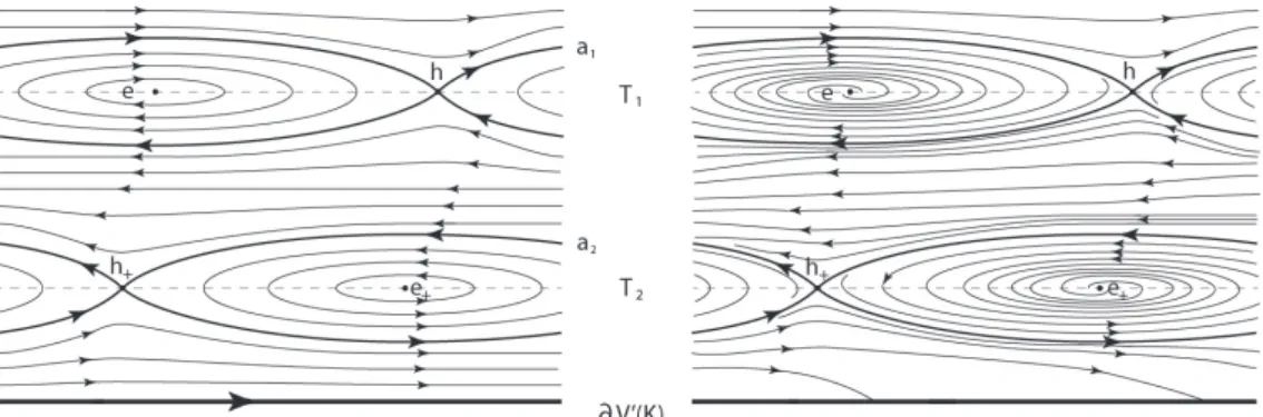
Note that the two bases of eigenvectors of LRh and LRh+ lie in the tangent spaces of the curves a1 and a2, respectively. We succeed in replacing the monomial representation of ρL([γ)] = [γ] given in Example 3.3.2 in the expression of the Lefschetz zeta function of Lemma 6.1.3. This is of course the degree of the (unique) orbit set in [γ]∼ that belongs to O(N3)and.

So for any ϑ0 such that P = (y0, ϑ0) is far from the curves in the diagram, there exists s0 ∈R such that u intersects Zs+. This degree is then different from the degree of the multisections of W+ counted by Φ (which is always 2g).

The generalization to links

The calculations will be done in terms of the Lefschetz zeta function of the ow of the Reeb vector part. To prove the above theorems we want to express the Euler characteristic χt1,..,tn(ECK(L, Y, α)) in terms of the twisted Lefschetz zeta function. Finally we let R0 =R in the rest of the manifold, where R was assumed to have only non-degenerate isolated periodic orbits.

Let us begin with the local Lefschetz zeta function of the simple trajectories (see Denition 3.3.3). It is interesting to note that the Euler characteristic of ECK1(L, Y, α) with respect to the surface S (see example 5.2.11) coincides with the sum of the Lefschetz signs of the Reeb trajectories in period 1 in the interior of S, i.e.

The general case

• Preliminary
• Proof of the results
• Monodromy and contact form near the binding
• ECH d for open books adapted to the binding
• Holomorphic curves near ∂N
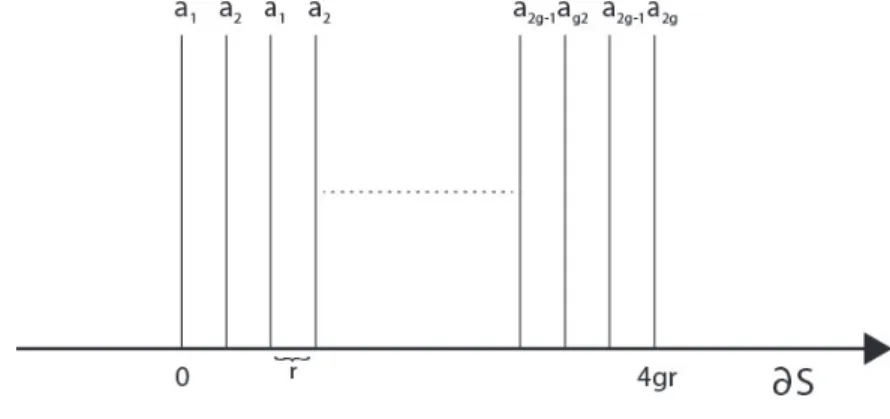
• The knot ltration inside the open book

From now on (Y, ξ) will be a contact 3-manifold and K ⊂ Y an oriented curved knot that is the bond of the open book decomposition (S, φ) of Y compatible with ξ, where S of xed is genusg. Moreover, condition 5 above implies that the behavior of the monodromy and the contact form near ∂Ne is the same as near ∂N. On the other hand, we decided to call them the same because they will play a somewhat analogous role in the definition of the node ltration.

For the same reason, all other leaf cylinders are of the ECH 2 index and are not numbered. By defining the ltering of the node, the Alexander degree will be given by the degree of the orbits as in Denition 2.2.9.

HFK d on a page

• The knot ltration on the page
• The homology

Note that the last definition can be seen as an analogue for the chord set of equation 7.1.13 for sets of orbits. Note that the setting ew is different from that in Section 4.1, but since they are in the same connected component of Σ\(β∪α), both choices give the same constraints on holomorphic curves counted by HF- differential. This result is analogous to equation 3.2.4 and can be recovered using the fact that the ltration given by deg is just a translation of the Alexander ltration, for which the result holds.

Since the set of the branching points ofuis nite, up to easily push K0 in their direction, by theorem. Since the signs of the intersections in equation 7.2.4 are all positive, ∂HF respects the ltration given by you.

Φ and the degree ltrations

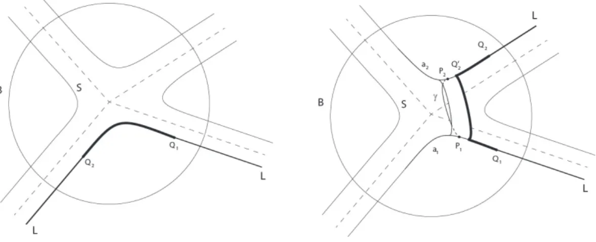
• Properties of the Φ -curves near ∂ S
• Φ is ltered

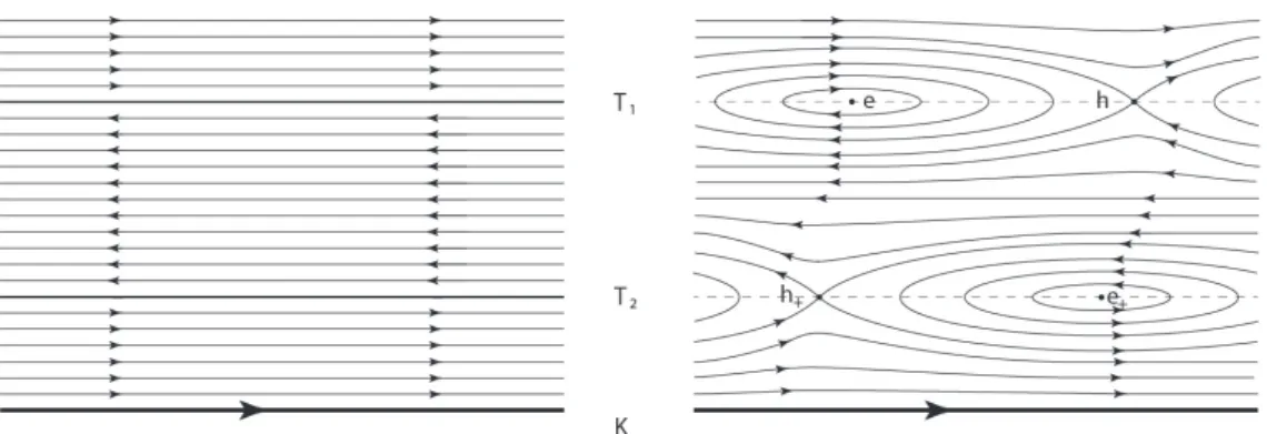
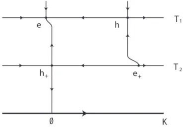
These maps are all isomorphisms: we will continue to call ([µ],[λ]) the preimages of the generators of H1(N{y∈[0,4]}) in each of the above groups. So far we have only made assumptions about the h−, e+, and h+ orbits, requiring that they be far from the curves of the diagram. Indeed, since ϑh− is far from the curves, the only possibility is that u0 contains a Morse function ow trajectory associated with T2 due to some chords in the direction of ϑh−.

This is not possible due to the fact that e+ is far from the curves and h+ is the minimum of the Morse function of T2 and close to the curves of the diagram. Before giving the last part of the proof of Theorem 7.3.8, we need a final lemma, the proof of which is very similar to that of Lemma 2.4.3 (avoiding considerations about the positivity of intersections).