l’élasticité de l’ADN

La chaîne étant plus rapide que la diffusion des « bras » (segments d’ADNdb qui entourent la bulle des deux côtés), la fermeture de la bulle se fait en rapprochant les deux bras jusqu’à ce que l’ADN adopte une conformation en épingle à cheveux. Nous avons montré que la dynamique de torsion joue un rôle primordial dans la fermeture des bulles de dénaturation, qui se produit là encore en deux étapes.

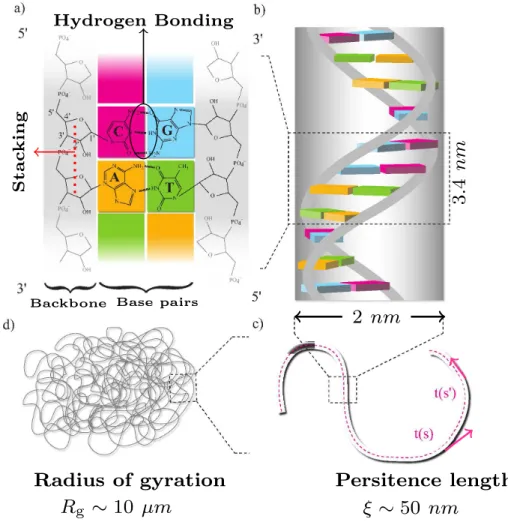
Structure of DNA

The stacking interactions arise mainly from the π−π interactions between the base aromatic rings along each ssDNA, as outlined in Figure 1.3. The flexibility of DNA on intermediate length scales can be described by the persistence length found in the Worm Like Chain (WLC) polymer model [9, 10] as shown in Figure 1.2c.

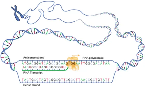
DNA functions

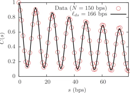
The persistence length is defined as the length over which the orientation vectors decorrelate, ˆt(0)·ˆt(s) =e−s/`p, where the orientation vectors, ˆt(0) and ˆt(s) are the tangent vectors of the average dsDNA chain. The initiation step corresponds to the identification by the RNA polymerase of the promoter region of the gene and its binding to it.

Figure 1.4: Sketch of RNA polymerase decoding the sequence and leaving behind the RNA transcript 1

DNA Denaturation

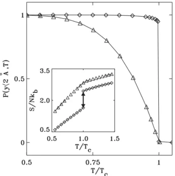
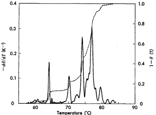
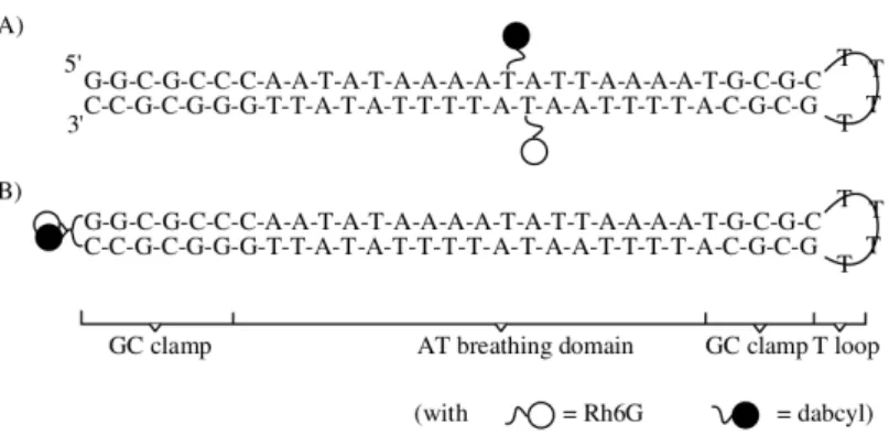
When the base pair is closed, the fluorophore is near the quencher and inhibits fluorescence. Note that at room temperature the probability of a bubble forming is almost zero.

Figure 1.6: Melting profile of pNT1 DNA, showing the cumulative profile (dotted line) and differential melting profile (solid line)

DNA Denaturation: Equilibrium

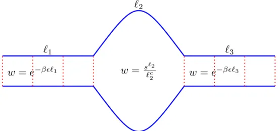
Poland-Scheraga model

The value of the loop exponent can be estimated using the random walk configurations, and it was found that for a phantom flexible loop, c = d2, where d is the spatial dimension. The value of cin in this case becomes,dν, where ν is Flory's exponent, which still makes the transition continuous in 2 and 3 dimensions.

Figure 1.8: A sketch of a DNA with bound segments of length, ` 1 , ` 3 and unbound segment of length, ` 2

Palmeri-Manghi-Destainville (PMD) model

DNA Denaturation: Dynamics

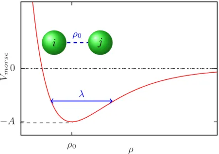
Peyrard-Bishop model
Barbi-Cocco-Peyrard model
Kim-Jeon-Sung model
Metzler et al. model

In this model, the torsional degrees of freedom of the base pairs are also relaxed. Duplex helicity and sequence effect are neglected in this model.

Figure 1.9: Sketch of model DNA showing the hydrogen interaction term and stacking term between the bases.

Bubble Dynamics: Experiments

The flexibility or stiffness of the polymer chains is controlled by the bending angle potentials. The strength of the potential κθ is related to the persistence length `p of the polymer as described in Chapter 1.

Figure 1.14: Sketch of M 18 DNA constructs: (A) with internal fluorescent tagging;

Overview of Coarse-Grained models of DNA available in the literature

Two beads per nucleotide

The model predicts sharp melting profiles but slow melting kinetics (a complete melting transition for 100 bps of DNA occurs only after 10 ns). Model parameters for hydrogen bonds and excluded volume interactions also depend on the sequence. The model is tested for a number of duplex decamers by comparing denaturation profiles with experimental ones.

The model consists of two beads per nucleotide, P for phosphate and sugar; B for the base, as shown in Fig.

Figure 2.4: Schematic representation of the model DNA by Zhang and Collins [60].

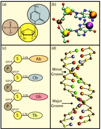
Three beads per nucleotide

The model captures the DNA pitch, the major and minor grooves of DNA as well. The size of the beads represents the range of excluded volume interactions. c)12 bp DNA as suggested by the model. The model correctly reproduces the experimental melting curves and the salt dependence of thermal melting.

The model gives a persistent length of ssDNA of 2 to 5 base pairs and dsDNA of 125 bps.

Figure 2.7: Schematic coarse-graining procedure for dsDNA. (a) Grouping of atoms.

Ladder DNA Model

Most of the models defined above are computationally expensive to achieve time scales of the order of µs or large DNA molecules. The first article of rhs. 2.19) is the stretching energy with the stretching modulus βκs = 100 (β−1 =kBT0, where T0 is room temperature) and a0 = 0.34 nm is the bead diameter and the equilibrium distance between two beads in each thread. The second term is the normal bending energy with a bending modulus κb,j that depends on the local chain configuration, as in the Kim-Jeon-Sung model described in Chapter 1.

We checked the equilibrium properties such as the persistence lengths of ssDNA and dsDNA, which are close to 3 bps and 150 bps, respectively.

Helical Model

Drawbacks of previous models

We expect that the denaturation dynamics depend on the values of persistence lengths of dsDNA`ds and ssDNA`s. To study the closure dynamics of the denaturing bubbles, the model DNA must have values of persistence lengths that are experimentally relevant. Most of the coarse-grained models of DNA lack acceptable values for either `ds or `ss.

The coarse-grained model developed by Knotts et al [58] results in `ds' of 60 bps which is less than the current value of 150 bps.

Equilibrium properties

An extension of the same model by Sambriski et al [68] leads to a good persistence length of dsDNA, `ds' 150 bps, but it lacks the good value for ss '36 bps. In this case the persistence length is purely the result of angular bending potential which is controlled by both κθ and θ0 since there is no torsional potential in ssDNA. 2.13, the persistence length of ssDNA is estimated by fitting the tangent-tangent correlation function at short distances with exp(−s/`ss).

It is possible to change the persistence length of ssDNA in our model, but then one must relax the dsDNA pitch.

Figure 2.12: The correlation function C(s) obtained for N = 150 bps dsDNA (The solid line is a fit from Eq

Numerical scheme

With a limited number of parameters in the model, we therefore chose a parameter set that leads to values of equilibrium parameters comparable to experiments, in contrast to the other models presented in this chapter. In the high friction limit, one can use the inertia term of Eq. 2.31) can be integrated numerically using the simple Euler's scheme. The value of ∆t should be chosen small as it can create instabilities in the simulations.

At the same time, ∆t should be greater than the pulse relaxation time τm, since we are dealing with an over-damped situation.

Summary

Brownian dynamics simulations

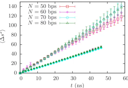
We studied the closure dynamics of a pre-equilibrated bubble in dsDNA using the ladder model 2.3, defined in Chapter 2. We created the bubble by turning off the Morse potential between strands and clamping the first and last three base pairs to create the full opening to prevent. of dsDNA. The initial bubble of size L(0) = N −6 was created in the center of a homopolymer DNA of N bps.

During closure, the first three base pairs on each side of the initial bubble are kept closed by applying an inter-strand attractive potential of 100 kBT, to prevent complete opening on both sides of dsDNA.

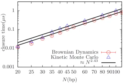
Kinetic Monte Carlo simulations

Closure dynamics

Fast zipping process

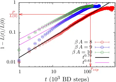
The unlocked part of the bubble is compared to the unadsorbed part of the polymer. In Fig.3.7b, the average size of the denatured part of DNA in renaturation and the bubble size in bubble closure are plotted, and we found the same scaling exponents. As the bubble size during zipping reaches the size of the persistence length of the ssDNA,. ss the bending force begins to compete with the driving force.

In a simple case of a circularly bent bubble, ¯ Ebend =κss4π2/4 ¯L=π2κss/L.¯ The size of the metastable bubble becomes, ¯L=p.

Figure 3.4: The averaged bubble size (normalized), L(t)/L(0) for N = 100 bps and for different Morse potential depths is shown with time

Metastable state

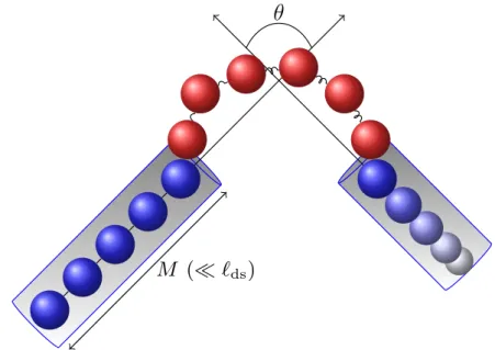
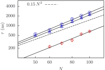
We plotted the dwell time and total closure time with M and N, respectively, as shown in Figure 3.12. So the dwell time is the mean first pass time, τmet(r|r0), for the pass from r0 to r, where r0 = (θ0, R0) and r = (θ, R), namely θ is the angle between the arms and R is the end-to-end distance of the bubble as schematically shown in the figure. The rotational diffusion of arms can be seen as a particle diffusing over a spherical surface.

The residence time distribution becomes broader and the average value increases for smaller κss values.

Figure 3.10: Sketch of two stiff rods connected by a flexible polymer.

Discussion

The above models also did not account for conformational degrees of freedom, which we have shown to play a key role in equilibrated bubble closure. The gap between these time scales may be due to the missing helicity in the current model. The bubble closes via two phases, a zipper and a metastable state, as in the previous ladder model.

Arm Diffusion Limited closure, limited by the alignment of the two arms by rotational diffusion as in the previous model.

Bubble closure dynamics

Zipping regime

As the bubble size reaches the order of persistence length of ssDNA, `ss, the bubble size starts to saturate and eventually stops closing further, leading to the metastable bubble of size ¯L. The torque Tbend(t) comes from the bending energy of two ssDNAs in the bubble and only plays a significant role when the two ssDNAs are stiff enough. Once the bubble size reaches the order of the persistence length of ssDNA, the torque Tbend plays a role.

As the size of the bubble decreases, the size of the arm thus increases. increasing the rotational friction of the wings.

Figure 4.3: The bubble size normalized by initial bubble size L(0) against time for βκ φ = 300

Metastable regime

From Fig.4.8 it is also clear that the bubble closes systematically by opening one end of the DNA. This is because the spreading of the bubble along the DNA is only a local phenomenon. However, the diffusion of the bubble along the DNA is limited by the alignment of the arms.

This cooperative nature in further closing of the bubble is the reason for the metastable state.

Figure 4.7: Sketch of the model DNA going through zipping with driving torque, T acting at each end of the bubble in opposite directions

Three different closure mechanisms and “Phase diagram”

Arms Diffusion Limited closure
Bubble Diffusion Limited closure
Temperature Activated closure
Classification of the three regimes

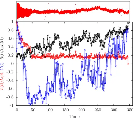
In Figure 4.1, by looking at ˆni·nˆe(t), the closure of the bubble for βκφ = 200 and N = 60 bps is limited by the rotational diffusion of the arms and occurs once the arms are nearly aligned. Figure 4.10 plots the MSD of the bubble along the DNA for different values of N. Although the ADL residence time is smaller compared to that of the BDL residence time, it can explain the different exponents.

BDL retention time or TA retention time is the time required for the DNA to completely close the vesicle either by opening at one end of the vesicle.

Figure 4.15: Log-log plot of BDL dwell ( 4 ) and closure times ( ◦ ) (βκ φ = 300), and ADL dwell times ( 3 ) (βκ φ = 200) with fitted laws

Discussion

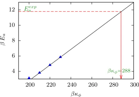
4.27, we have indicated the estimated torsional constant in the phase diagram of the two mechanisms of closure. Apart from the radial coordinate, as in the PB model, an angular coordinate is also included in this model. These models also lack the chain degrees of freedom and the distribution of the entire chain in space, which have been shown to play a crucial role in the closure of denaturation bubbles using the ladder model.

However, as already discussed previously, this model lacks the flexibility of whole DNA and single-stranded DNA, which we have shown to play an important role in the activation energy barrier.

Figure 4.26: Activation Energy is plotted against κ φ for N = 70 bps. The black line is a linear fitted law and it is extrapolated to experimental activation energy,

Perspectives

that the elasticity of DNA plays an important role in DNA denaturation at an equilibrium level. The accurate mapping will lead to a better understanding of the zipper dynamics in the bubble closure in the ladder model. The helical model is not limited to the exploration of bubble closure dynamics, but can be used to study, for example, mechanical denaturation of DNA.

To compare it with the chain dynamics in bubble closure, we also studied the hybridization (or renature) dynamics of helical DNA.