Given the unique continuation property (5), the map ϕT 7→ kϕTkH is a Hilbert norm in D(Ω). Point (ii) is a consequence of the symmetry and positivity of the bilinear form aε. But this means that λε∈L2(QT) is a solution of the heat equation in the transposition sense.
The equivalence of the mixed formulation (26) with the mixed formulation (16) is related to the regulation property of the heat wick. The solutionϕ of the mixed formulation (32) belongs to Wfρ0,ρ and therefore does not depend on the weight ρ (remember that ρ is strictly positive); this is consistent with the fact that ρ does not appear in the original formulation formulation (29).
Discretization of the mixed formulation (16)
Therefore, this weight can be seen as a parameter to improve some specific properties of the mixed formulation, specifically at the numerical level. Precisely in the limiting case ε= 0, we remember that traceϕ|t=T of the solution does not belong to L2(Ω), but to a much larger and single space. Note that this is actually the effect and role of the Carleman type weights, defined by (33) and originally introduced in [21].
As in Section 2.1, it is convenient to "augment" the Lagrangian and instead consider the LagrangianLr defined for anyr >0 with. Then we can introduce the following approximate problems: find (ϕh, λh)∈Φε,h×Mε,hsolution. 40) The well-placedness of this mixed formulation is again a consequence of two properties: the coercivity of the bilinear formaε,ron subsetNh(b) ={ϕh∈Φε,h;b(ϕh, λh) = 0 ∀λh∈ Mε ,h}. For any fasth, the spaces Mε,hand Φε,have of finite dimension, so that the infimum and supremum in (41) are reached: moreover, from the property of the bilinear formaε,r, it is standard to prove that δh is strictly positive ( see section 3.3).
On the other hand, the property infhδh>0 is generally difficult to prove and strongly depends on the choice made for the approximated spaces Mε,h and Φε,h. In the one-dimensional setting discussed below, there are 16 degrees of freedom, namely the values of ϕh, ϕh,x, ϕh,t, ϕh,xt at the four vertices of each rectangle K. On the other hand, the matrix is of order mh+nh in (42) is symmetric but not positive definite.
To evaluate the matrix coefficients, we use the exact integration methods developed in [14].
Normalization and discretization of the mixed formulation (32)
We also mention that the approximation is conformal: for every h >0, we have Φε,h⊂Φεand Mε,h⊂L2(QT). The matrix Aε,r, also has the symmetric and positive definite measure matrix Jhare for anyh >0 and every r > 0. Let us also mention that forr = 0, although the formulation (16) is well positioned, numerically, the corresponding matrix Aε ,0, h is not reversible according to remark 2.
The corresponding controlled state yε,h can be obtained by solving (1) with standard forward approximation (we refer to [10], Section 4 where it is detailed). Here, since the controlled state is given directly by the multiplierλ, we simply useλ has an approximation of y and do not report here the calculation of yh. Each element is a rectangle of lengths ∆x and ∆t; ∆x >0 and ∆t >0 denote, as usual, the discretization parameters in space and time respectively.
Moreover, the optimal controlled state is still given by ρ−1λ, while the optimal control is expressed in terms of the variable ψasv=ρ−10 ψ1ω. The corresponding discretization approach (completed with the termrkρ−1L⋆(ρ0ψ)kL2(QT)) is as follows: find (ψh, λh)∈Φh×Mhsolution of. In this respect, the change of variable can be seen as a precondition for the mixed formulation (32).
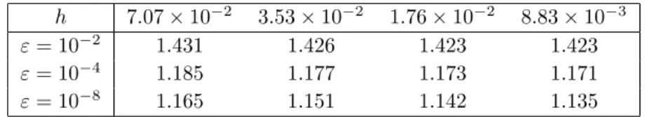
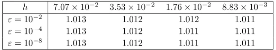
The discrete inf-sup test
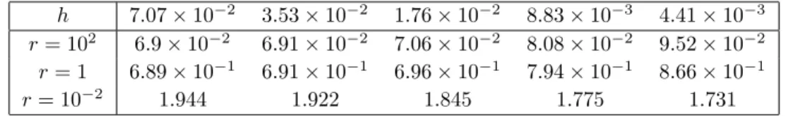
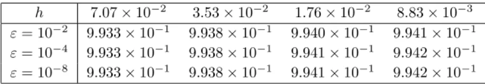
We now give some numerical values of δε,r,h with respect to h for the C1-finite element presented in Section 3.1. We also note that for sufficiently large (see Tables 2 and 3) the value of the inf-sup constant is almost constant with respect to ε and behaves similarly. More importantly, we note that for any r and ε the value of δε,r,h is bounded below uniformly with respect to the discretization parameter h.
The same behavior is observed for other discretizations, so that ∆t 6= ∆x, different supports ω and different choices for the weightρ0 (in particular ρ0:= 1). Consequently, we can conclude that the finite approximation we used 'passes' the discrete inf-sup test. It is interesting to note that this is in contrast to the situation for the wave equation which requires careful adjustment of the parameter r with respect to toh; we refer to [11].
Moreover, as is common in mixed finite element theory, such a property together with the uniform constraint of formaε,r implies the convergence of the approximation sequence (φh, λh) solution of (40). Similarly, Table 4 shows the discrete constant of inf-sup corresponding to the limiting case of. Again, for the limiting case, the value given in the Table suggests a similar behavior observed for ε >0: the constant is bounded uniformly from below with respect to the hand parameter behaves more -1/2 for enough (up to 1 ).
Note that, due to the introduction of the weightρ6= 1, the inf-sup constants given by Table 4 are not the limit (asε→0) of the previous Tables.
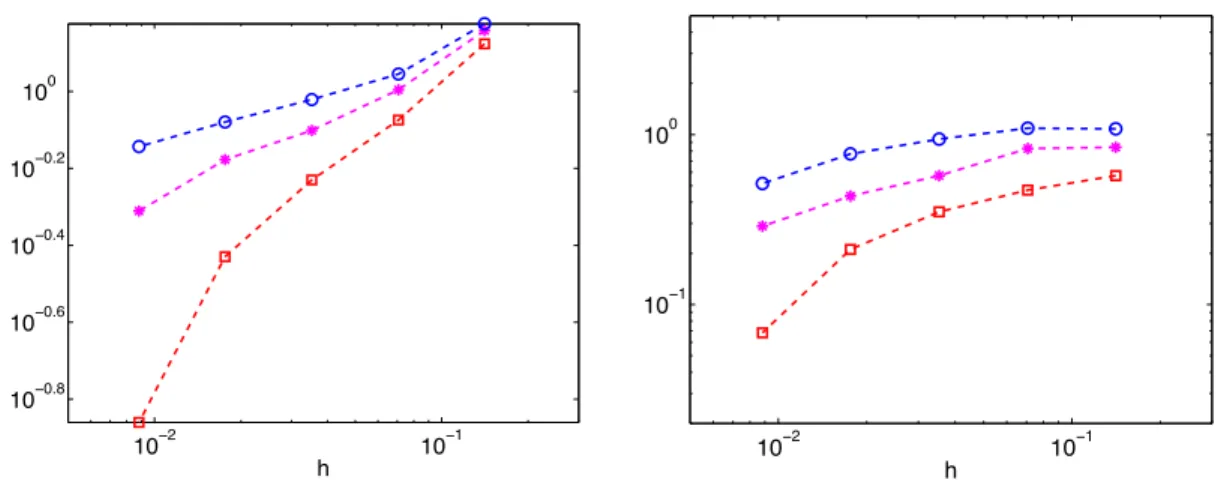
Numerical experiments for the mixed formulation (16)
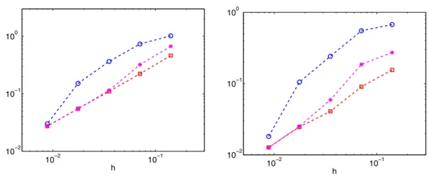
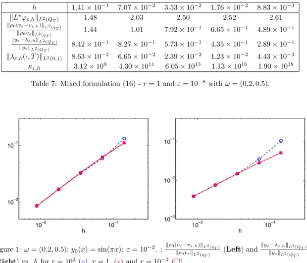
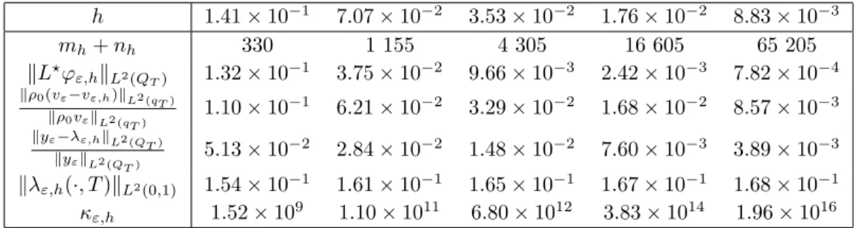
We then check convergence, since h tends to zero of the approximations (vε,h, λε,h) towards the optimal pair (vε, yε) in L2(qT)×L2(QT) for all values of εandr. More precisely, for a sufficiently large value of ε (here ε = 10−2), we observe a quasi-linear convergence rate for both kρ0(vkρε0−vv ε,h)kL2(qT). For small values of ε, we observe reduced convergence, both for the control and for the condition (see Figure 2 for ε= 10−4 and Figure 3 for ε= 10−8).
We recall that if it is zero, the space Φε degenerates into a much larger space and oscillates very close to T. This does not prevent the convergence of the variable ϕε,h for the norm Φε, in particular the control vε,h =ρ−2ϕε,h1ω , and of the variable λε,h. We will return to this situation in detail in the section on the limiting case = 0.
Moreover, for small value of ε, the parameters have influence; precisely, a low value ofr(herer= 10−2) leads to better relative errors: this is consistent with the behavior of the constant inf-supδ,r,h which increases with r−1/2. Remarkably, we note that the variational approach developed here allows, for any ε, a direct and robust approximation of a control for the heat equation. As discussed extensively in [19, 34], the minimization of the conjugate function Jε⋆ using the conjugate gradient algorithm requires a number of iterations for small ε (typically ε= 10−8 and ω and diverges for small values ofh.
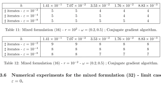
Conjugate gradient for J ε,r ⋆⋆
As described in detail in [19, 34], the minimization of the conjugate functional Jε⋆ using the conjugate gradient algorithm requires a number of iterations for smallε (typically ε= 10−8 and ω and diverges for small values of iii) Test of convergence and construction of the new descent direction Updategεn city. From the previous estimate, the performance of the algorithm related to the condition number of the operator Aε,r is limited to Mε,h ⊂ L2(QT), which here (see [4]) coincides with the condition number of the symmetric and positive definite matrix BhA−1ε,r ,hBTh introduced in (46). Consequently, the condition number is expressed in terms of the margin of the discrete inf-sup constantδε,h as follows.
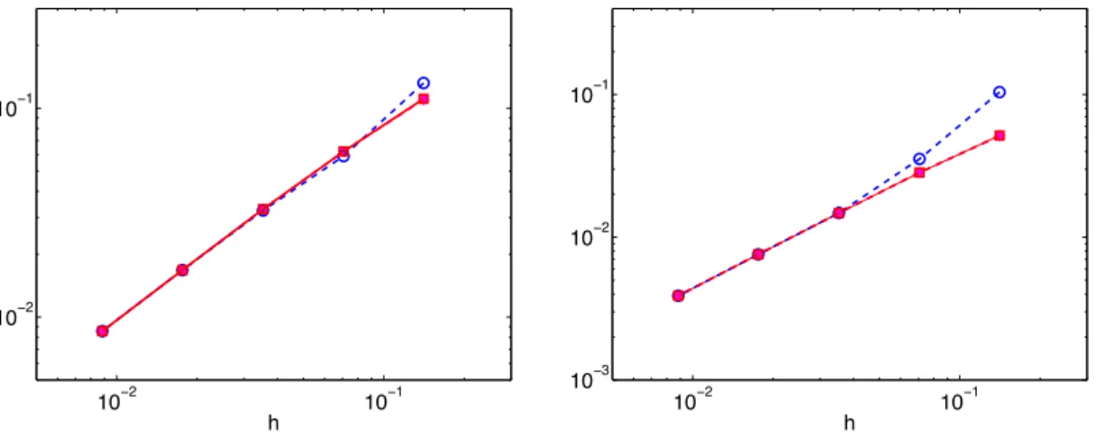
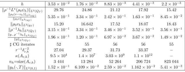
Since the discrete inf-sup constantδε,r, from our observation in Section 3.3, is uniformly bounded below with respect to toh, we deduce that the condition number is uniformly bounded by above with respect to the discretization parameter. This implies that the convergence of the sequence {λnε,h}(n>0), minimizes forJε,r⋆⋆ overMε, its independent ofh. We check that the method provides, for the same value of r, ε and h, exactly the same approximation λε,h as the previous direct method (see Tables 5, etc.).
This again contrasts with the behavior of the conjugate gradient algorithm when the latter is used to minimize Jε⋆ with respect to ϕT defined by (13). According to this very low number of iterations, it seems more advantageous not only in terms of memory resources, but also in terms of time execution to solve the extreme problem in the variable λε than the (equivalent) mixed formulation (40). Note, however, that the condition number of the matrix Aε,r,his is not independent of h, but behaves polynomially (see Table 10 where the value is reported for r = 1).
On the other hand, the number of conditions decreases slightly with (recall that the norm over Φε.
Numerical experiments for the mixed formulation (32) - limit case ε = 0
This high robustness of the approach definitively contrasts with the classical dual methods discussed in [34] and the references therein: We recall that for ε = 0, the minimization of Jε=0⋆ defined by (13) fails when it is small enough is. In particular, the smallness of both the diffusion coefficient and the magnitude of the support w leads to a large amplitude of control at the initial time. The experiments reported here - in the borderline case ε = 0 - were obtained for a specific choice of the weights ρ0 and ρ.
This allows in particular to avoid the high oscillatory behavior of the minimumL2-rate control, which is when ρ0 := 1 in qT. The exponential behavior of the control implies a similar behavior of the corresponding controlled statementρ−1λ, so the choice of parameterρ made here is also natural. The mixed formulation we have introduced here to handle the zero controllability of the heat equation seems original and has adapted the work [11] devoted to the wave equation.
The main ingredients that allow the mixed formulation to prove well-posed are an observability inequality and a direct inequality (usually derived from energy estimates). It is worth mentioning that within this mixed formulation approach, the strong convergence of the approximations (as achieved within a closed but different approach by [18] assuming that the weights ρ0 and ρ coincide with the Carleman weight) must still be performed. . We use the characterization of the pair (yε, vε) in terms of the adjoint solutionϕε(see (5)), unique minimization iL2(Ω) of Jε⋆ defined by (13).
The resolution of the infinite dimensional system (reduced to a finite dimension one by truncation of the sums) allows an approximation of the minimizerϕT,ε ofJε⋆.
Appendix: Tables
M¨unch, Numerical controllability of the wave equation using primal methods and carleman estimates, ESAIM Control Optim. M¨unch, Mixed formulation for direct approximation of minimum L2-norm control for wave equations of linear type, Appears in Calcola (http://hal.archives-ouvertes.fr/hal-00853767). M¨unch, Numerical null controllability of semilinear 1-D heat equations: fixed point, least squares and Newtonian methods, Math.
19] ,Numerically exact controllability of the 1d heat equation: Carleman weights and duality, Journal of Optimization Theory and Applications, (2014). 34 of Lecture Notes Series, Seoul National University Research Institute of Mathematics Global Analysis Research Center, Seoul, 1996. Lions, Exact and approximate controllability for distributed parameter systems, in Acta numerica, 1995, Acta Numer., Cambridge Univ.