[PENDING] Modèles et algorithmes pour la simulation du contact frottant dans les matériaux complexes : application aux milieux fibreux et granulaires

HAL Id: tel-01684673

https://tel.archives-ouvertes.fr/tel-01684673

Submitted on 15 Jan 2018

HAL is a multi-disciplinary open access archive for the deposit and dissemination of sci- entific research documents, whether they are pub- lished or not. The documents may come from teaching and research institutions in France or abroad, or from public or private research centers.

L’archive ouverte pluridisciplinaire HAL, est destinée au dépôt et à la diffusion de documents scientifiques de niveau recherche, publiés ou non, émanant des établissements d’enseignement et de recherche français ou étrangers, des laboratoires publics ou privés.

frottant dans les matériaux complexes : application aux milieux fibreux et granulaires

Gilles Daviet

To cite this version:

Gilles Daviet. Modèles et algorithmes pour la simulation du contact frottant dans les matériaux complexes : application aux milieux fibreux et granulaires. Algorithme et structure de données [cs.DS].

Université Grenoble Alpes, 2016. Français. �NNT : 2016GREAM084�. �tel-01684673�

Pour obtenir le grade de

DOCTEUR DE L’UNIVERSITÉ DE GRENOBLE

Spécialité :Mathématiques-informatique

Arrêté ministériel du 25 mai 2016

Présentée par

Gilles Daviet

Thèse dirigée parFlorence Bertails-Descoubes

préparée au sein de l’équipe-projet Bipop, Inria et Laboratoire Jean Kuntzmann et de l’école doctorale “Mathématiques, Sciences et Technologies de l’Information, Informatique”

Modèles et algorithmes

pour la simulation du contact frottant dans les matériaux complexes

Application aux milieux fibreux et granulaires

Thèse soutenue publiquement le15 décembre 2016, devant le jury composé de :

Dr Georges-Henri Cottet

Professeur des universités, Université Grenoble Alpes, Président Dr Robert Bridson

Adjunct Professor, University of British Columbia et

Senior Principal Researcher for Visual Effects, Autodesk, Rapporteur Dr Ioan Ionescu

Professeur des universités, Université Paris 13, Rapporteur Dr Jean-Marie Aubry

HDR, Visual Effects Researcher, Double Negative Visual Effects, Examinateur Dr Pierre-Yves Lagrée

Directeur de recherche, Institut d’Alembert, CNRS, Examinateur Dr Pierre Saramito

Directeur de recherche, Laboratoire Jean Kuntzmann, CNRS, Examinateur Dr Florence Bertails-Descoubes

En premier lieu, je tiens bien sûr à remercier les rapporteurs et examinateurs de cette thèse, en particulier pour leur patience quand à la lecture de ce manuscrit — qui, reconnaissons le, com- porte quelques sections pouvant s’avérer arides. Je remercie également le labex PERSYVAL-Lab¹ de m’avoir octroyé la bourse m’ayant finalement permis d’effectuer cette thèse, après une demi- douzaine de refus auprès d’organismes variés — et évidemment, Florence et Pierre, pour ne pas avoir désespéré malgré lesdits refus. Merci en outre à Pierre pour m’avoir initié à la simulation des fluides complexes, et Florence, pour m’avoir recueilli tout fraîchement sorti de l’Ensimag et m’avoir donné goût à ce domaine bien spécifique de l’animation pour l’informatique graphique, puis m’avoir porté en tant qu’ingénieur de recherche et doctorant. Je remercie l’équipe Bipop et l’Inria de m’avoir accueilli près de six ans, et tous ceux, permanents ou non-permanents, que j’ai pu rencontré dans ce cadre, et qui m’ont transmis quelques intuitions quand à la mécanique du contact, l’optimisation, ou d’autres sujets moins scientifiques. Merci en particulier aux précé- dents doctorants de Bipop et de la Tour pour leur rôle de modèles exemplaires : Florent, dont le manuscrit aura été une source d’informations inestimable ; Alexandre, Romain, Sofia, mes co-bureaux m’ayant préparé à la Rédaction, vraisemblablement avec succès. Merci également à mes anciens collègues de Weta Digital, qui ont largement contribué à élargir mes horizons culturels et scientifiques.

Car cette thèse n’aurait pu s’achever sans les moments de détente qui l’ont entrecoupé, je remercie les InuIts (et apparentés) pour les sorties à Grenoble et ailleurs, les randonnées et autres bivouacs — et parmi eux mes illustres prédécesseurs thésards, pour m’avoir encouragé à continuer dans cette voie et pour la richesse de leurs discussions, en particulier en fin de Fam’s.

Finalement, je remercie ma famille, non seulement pour son support inconditionnel mais pour avoir initié ma curiosité scientifique et mon goût pour la programmation (à travers le GW- BASIC !), sans lesquels je n’aurais sans doute jamais entrepris de telles études. Plus que tout, merci à Anaïs, qui m’aura supporté et encouragé tout au long de cette thèse, et m’aura accom- pagné au bout du monde.

1This work has been partially supported by the LabEx PERSYVAL-Lab (ANR-11-LABX-0025-01) funded by the French program Investissement d’avenir

Remerciements 3

Contents 5

Nomenclature 11

Introduction 15

0.1 Motivation . . . 15

0.1.1 Granular materials . . . 15

0.1.2 Dynamics of hair and fur . . . 16

0.1.3 Target applications . . . 16

0.2 Contacts and dry friction . . . 18

0.2.1 Impacts . . . 18

0.2.2 Dry friction . . . 19

0.2.3 Other friction laws . . . 20

0.2.4 Discrete simulation of complex materials with frictional contacts. . . 22

0.3 Continuum modeling of dry friction . . . 23

0.3.1 Yield-stress flows . . . 23

0.3.2 Frictional yield surfaces . . . 23

0.3.3 Shearing granular flows . . . 25

0.3.4 Other complex materials. . . 26

0.4 Synopsis . . . 26

I Numerical treatment of friction in discrete contact mechanics 29 1 Mathematical structure of Coulomb friction 31 1.1 Coulomb’s friction law. . . 31

1.1.1 Second-Order Cone. . . 31

1.1.2 Disjunctive formulation of the Signorini-Coulomb conditions . . . 32

1.1.3 Alart–Curnier function . . . 33

1.2 Implicit Standard Materials. . . 34

1.2.1 Generalized Standard Materials . . . 34

1.2.2 Implicit Standard Materials . . . 35

1.3 Application to Drucker–Prager plasticity . . . 38

1.3.1 Symmetric tensors . . . 38

1.3.2 Drucker–Prager yield surface . . . 39

1.3.3 Dilatancy and non-associated Drucker–Prager flow rule . . . 40

1.3.4 Bipotential and reformulations of the Drucker–Prager flow rule. . . 41

1.3.5 Viscoplasticity . . . 44

2 Modeling contacts within the Discrete Element Method 47 2.1 A few mechanical models for rigid and deformable bodies in finite dimension . . 47

2.1.1 Rigid-body dynamics . . . 47

2.1.2 Lumped system . . . 51

2.1.3 Lagrangian mechanics . . . 52

2.1.4 Discussion . . . 54

2.2 Contacts . . . 55

2.2.1 Continuous-time equations of motion with contacts . . . 56

2.2.2 Time integration. . . 57

2.2.3 Collision detection . . . 60

2.3 Discrete Coulomb Friction Problem . . . 61

2.3.1 Reduced formulation . . . 61

2.3.2 Fixed-point algorithms and existence criterion . . . 62

3 Solving the Discrete Coulomb Friction Problem 67 3.1 Global strategies . . . 67

3.1.1 Pyramidal friction cone . . . 67

3.1.2 Complementarity functions . . . 68

3.1.3 Optimization-based methods . . . 69

3.2 Interior-point methods. . . 70

3.2.1 Second-Order Cone Programs . . . 70

3.2.2 Discussion . . . 71

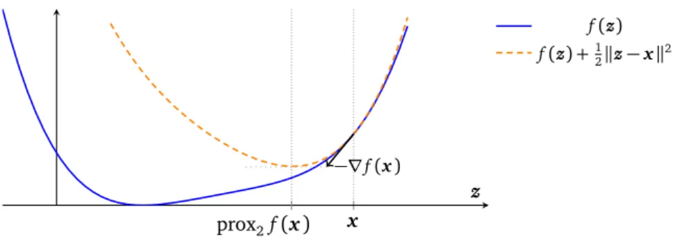
3.3 First-order proximal methods . . . 71

3.3.1 Proximal operator. . . 71

3.3.2 Projected Gradient Descent . . . 73

3.3.3 Primal–dual proximal methods. . . 74

3.4 Splitting methods . . . 78

3.4.1 Operator splitting . . . 78

3.4.2 Convergence properties . . . 79

3.4.3 Performance . . . 80

3.4.4 Discussion . . . 82

4 A Robust Gauss–Seidel Solver and its Applications 83 4.1 Hybrid Gauss–Seidel algorithm . . . 83

4.1.1 SOC Fischer-Burmeister function. . . 83

4.1.2 Analytical solver. . . 85

4.1.3 Full algorithm . . . 88

4.2 Application to hair dynamics . . . 89

4.2.1 Hair simulation in Computer Graphics . . . 91

4.2.2 Full-scale simulations. . . 92

4.2.3 Friction solvers comparisons . . . 94

4.2.4 Limitations . . . 97

4.3 Application to cloth simulation . . . 98

4.3.1 Nodal algorithm . . . 98

4.3.2 Results. . . 100

4.3.3 Limitations . . . 100

4.4 Inverse modeling with frictional contacts . . . 101

4.4.1 Linear case . . . 101

4.4.2 Nonlinear case . . . 103

II Continuum simulation of granular materials 107 5 Continuum simulation of granular flows 109 5.1 Continuum models . . . 109

5.1.1 Inelastic yield-stress fluids. . . 110

5.1.2 Elasto-plastic models . . . 111

5.2 Spatial discretization strategies . . . 112

5.2.1 Continuous conservation equations . . . 112

5.2.2 Mesh-based discretization . . . 113

5.2.3 Particle-based discretization. . . 115

5.2.4 Hybrid methods . . . 116

5.3 Our approach . . . 117

5.3.1 Design goals . . . 117

5.3.2 Outline of this second part . . . 118

6 Dense granular flows 119 6.1 Constitutive equations . . . 119

6.1.1 Unilateral incompressibility . . . 119

6.1.2 Friction . . . 120

6.2 Creeping flow . . . 122

6.2.1 Steady-state and boundary conditions . . . 122

6.2.2 Variational formulation . . . 123

6.2.3 Cadoux algorithm. . . 124

6.3 Discretization using finite-elements . . . 126

6.3.1 Discretization of the symmetric tensor fields . . . 126

6.3.2 Discretization of the (bi)linear forms . . . 128

6.3.3 Discretization of the Drucker–Prager flow rule . . . 128

6.3.4 Considerations onR^† . . . 131

6.3.5 Final discrete system . . . 132

6.4 Solving the discrete problem . . . 133

6.4.1 Discrete Cadoux fixed-point algorithm . . . 133

6.4.2 Dual problem . . . 134

6.4.3 Solving the minimization problems . . . 135

6.5 Results . . . 136

6.5.1 Model problems . . . 136

6.5.2 Flow around a cylinder. . . 139

6.5.3 Extension to inertial flows: discharge of a silo . . . 140

6.5.4 Performance . . . 143

7 Dry granular flows 149 7.1 Spatially continuous model . . . 149

7.1.1 Constitutive equations . . . 149

7.1.2 Energy considerations . . . 150

7.1.3 Semi-implicit integration . . . 152

7.1.4 Discrete-time equations . . . 153

7.2 Discretization using finite elements . . . 155

7.2.1 Space compability criterion . . . 155

7.2.2 Piecewise-constant discretization . . . 156

7.2.3 Results. . . 160

7.3 Material Point Method. . . 162

7.3.1 Application to our variational formulation. . . 163

7.3.2 Grid–particles transfers . . . 163

7.3.3 Shape functions . . . 165

7.3.4 Numerical resolution . . . 167

7.3.5 Overview of a time-step . . . 169

7.4 Extensions . . . 169

7.4.1 Rigid body coupling and frictional boundaries . . . 170

7.4.2 Anisotropy . . . 172

7.5 Results . . . 173

7.5.1 Model problems. . . 174

7.5.2 Complex scenarios . . . 176

7.5.3 Performance . . . 178

7.5.4 Limitations . . . 179

7.6 Discussion . . . 180

8 Granular flows inside a fluid 181 8.1 Related work. . . 181

8.1.1 Modeling . . . 182

8.1.2 Numerical simulations . . . 184

8.2 Two-phase model . . . 186

8.2.1 Base equations . . . 186

8.2.2 Stresses and buoyancy . . . 186

8.2.3 Drag force . . . 188

8.2.4 Mixture conservation equations . . . 189

8.2.5 Dimensionless equations. . . 191

8.2.6 Particular cases . . . 193

8.3 Numerical resolution of the two-phase equations . . . 195

8.3.1 Time discretization . . . 195

8.3.2 Variational formulation . . . 196

8.3.3 Discrete system . . . 197

8.3.4 Spatial discretization . . . 198

8.4 Results . . . 199

8.4.1 Rayleigh-Taylor instability. . . 199

8.4.2 Sedimentation . . . 199

8.4.3 Regimes . . . 200

8.4.4 Limitations . . . 202

8.4.5 Conclusion . . . 203

Conclusion 205 9.1 Key remarks and summary of contributions . . . 205

9.2 Perspectives . . . 206

Appendices 209 A Convex analysis 211 A.1 Operations on convex functions . . . 211

A.1.1 Fundamental definitions. . . 211

A.1.2 Subdifferential of a function . . . 211

A.1.3 Convex conjugate . . . 213

A.2 Normal and convex cones. . . 214

A.2.1 Normal cone . . . 214

A.2.2 Operations on normal cones . . . 215

A.2.3 Convex cones . . . 217

A.3 Constrained optimization . . . 218

A.3.1 Optimality conditions . . . 219

A.3.2 Lagrange multipliers . . . 220

B Discrete Coulomb Friction Problem solvers 227 B.1 Newton SOC Fischer–Burmeister function. . . 227

B.1.1 SOC Fischer–Burmeister derivatives. . . 227

B.1.2 Optimistic Newton algorithm . . . 228

B.2 Suggested variants of the Projected Gradient Descent algorithm . . . 228

B.3 Convergence of the out-of-order Gauss–Seidel algorithm. . . 229 C Supplemental justifications related to Drucker–Prager constraints 233

C.1 Constraints on quadrature points . . . 233

C.2 Frictional boundaries. . . 234

C.2.1 Signorini condition . . . 234

C.2.2 Tangential reaction . . . 234

C.2.3 Reverse inclusion . . . 235

Bibliography 237

Abstract – Résumé 252

Abbreviations

ADMM Alternating Direction Method of Multipliers (Section3.3.3) AMA Alternating Minimization Algorithm (Section3.3.3)

DCFP Discrete Coulomb Friction Problem (Section2.3) DEM Discrete-Element Modeling (Section0.2.4) FEM Finite-Element Modeling (Section5.2.2) FLIP FLuid-Implicit Particle method (Section5.2.4) GSM Generalized Standard Material (Section1.2.1) ISM Implicit Standard Material (Section1.2.2) MPM Material Point Method (Section5.2.4) NSCD Non-Smooth Contact Dynamics (Section3.4) PIC Particle-in-Cell method (Section5.2.4) SOC Second-Order Cone (Definition1.1) SOCP Second-Order Cone Program (Section3.2)

SOCQP Second-Order-Cone Quadratic program (Section2.3.2) SOR Successive Over-Relaxations (Section3.4.3)

DP Drucker–Prager (yield surface, Section0.3.2) MC Mohr–Coulomb (yield surface, Section0.3.2 Constants

Bi Bingham number Fr Froude number Re Reynolds number St Stokes number

d Dimension of the simulation space (usually 2 or 3) α (Chapter8only) Scaled density difference,α:=^ρg_ρ^−ρf

f

ε (Chapter8only) Ratio of scales,ε:=D_g/L

e_i i^thcomponent of the canonical basis of an Euclidean space I_n Identity tensor of dimensionn(nmight be ommitted)

ι_d Unit normal tensor for the scalar productS²_d→R,σ,τ7→ ¹₂·σ:τ·

s_d Dimension of the spaceS_dof symmetric tensors withdrows and columns,s_d=¹₂d(d+1)

Ω Simulation domain (for continuum mechanics) or rigid-body B_D Part of the boundary ofΩwith Dirichlet boundary conditions B_N Part of the boundary ofΩwith Neumann boundary conditions

∆t Timestep size

ζ Dilatancy coefficient (in the context of granular flows) η Dynamic viscosity

g Gravity vector µ Coefficient of friction

n Normal vector (for a given contact point) φ_max Maximal volume fraction

ρ Volumetric mass σ_S Shear yield stress τ_c Tensile yield stress c Cohesion coefficient

D_g Average diameter of the grains L Characteristic length

Differential operators

∇ ·τ Divergence of a vector or tensor fieldτ

∂f

∂x Partial derivative or subdifferential of a functionf w.r.t. a single varibalex

Dφ

Dt Total ormaterialderivative of a fieldφ, c.f. Section5.2.1

∇f Gradient of a function (or of a vector or scalar field)f

W(v) Skew-symmetric part of the gradient of a vector fieldv, W(v):= ¹₂∇v−¹₂(∇v)^⊺ D(v) Symmetric part of the gradient of a vector fieldv, D(v):= ¹₂∇v+¹₂(∇v)^⊺

∂f Subdifferential of a functionf (DefinitionA.6) Functions

IC Characteristics function of the setC(DefinitionA.8) δⁱ_j Kronecker delta

δ Dirac delta function

f_AC Alart–Curnier function, defined in Equations (1.6,1.27) f_BK Kynch batch flux density function, defined in Section8.1.1 f_DS De Saxcé function, defined in Equation (1.29)

f_DS Fischer–Burmeister function, defined in Section4.1.1 Mathematical operators

〈u,v〉 Dot product of vectorsuandv

τ:σ Twice-contracted tensor product. For rank-2 tensors,τ:σ=P

i,jτ_{i j}σ_ji τ⊗σ Tensor (outer) product ofτandσ

u∧v Cross product of 3D vectorsuandv

ΠC Orthogonal projection on a set (CorollaryA.6) M Mass or stiffness matrix

W Delassus operator

adj Adjugate matrix (transpose of cofactor matrix)

atan2 A two-arguments arctangent function that is robust to edge cases² L·M Average values of a field at a discontinuity

f^⋆ Convex conjugate of a function (DefinitionA.7) Conv Convex hull of a set

Dev Deviatoric (traceless) part of a tensor

diag (Block-)diagonal matrix obtained by diagonal concatenation of several coefficients or blocks

dom Effective domain of a function (DefinitionA.3) epi Epigraph of a function (DefinitionA.2) Im Image of a linear operator

relint Relative interior of a set

J·K Jump (difference in values) of a field at a discontinuity Ker Kernel of a linear operator

·N Normal part of a vector (w.r.t.n) or tensor (w.r.t.ι_d) C Closure of the setC

prox Proximal operator (Definition3.1)

Span Set spanned by linear combinations of a set of vectors

·T Tangential part of a vector (w.r.t.n) or tensor (w.r.t. ι_d) Tr Trace of a tensor

Bd Boundary of a set int Interior of a set

I₁(σ) First invariant of a tensorσ,I₁(σ):=Trσ

J₂(σ) Second invariant of the deviatoric part of a tensorσ,J₂(σ):=Trσ² Sets and spaces

Kµ Second-Order Cone (SOC) of apertureµ(Definition1.1)

Tµ,σS Truncated SOC of apertureµand base sectionσ_S(Section1.3.2)

H¹(Ω) Sobolev spaceW^1,2 of square integrable functions with square-integrable derivatives over a domainΩ

H₀¹(Ω) Subspace ofH¹(Ω)satisfying homogeneous Dirichlet boundary conditions L₂(Ω) Space of square integrable functions over a domainΩ

T_h⊂L₂(Ω)^sd Discrete space of symmetric tensor fields

2Seehttps://en.wikipedia.org/wiki/Atan2

V_h(0)⊂H₀¹(Ω)^d Discrete space of velocity fields [a,b]⊂R Closed interval

]a,b[⊂R Open interval

NC Normal cone to a setC(DefinitionA.9) K^◦ Polar cone to a setK(DefinitionA.11)

Cµ Set of velocity–force solutions to the Signorini–Coulomb frictional contact law (Sec- tion1.1.2)

DP Set of strain–stress solutions to the non-associated Drucker–Prager rheology (Section1.3.3) R¯ R∪ {−∞,+∞}

Variables (discrete mechanics)

λ Lagrange multipliers associated to holonomic constraints q Generalized coordinates

r Contact reaction forces

u Relative velocities of contacting objects

˜

u Relative velocities afterde Saxcéchange of variable (Section1.2.2) v Generalized velocities

Variables (granular flows)

β Scaled mass field,β:=αφ+1

˙

ǫ Strain rate tensor, ˙ǫ:=D(u) ǫ Strain tensor

η_eff Effective viscosity field

γ Affine combination of the strain rate tensor with positive divergence λ Opposite of contact stress tensor

φ Volume fraction field

π Product fraction field,π:=φ(1−φ) σ Stress tensor

u Velocity field ξ Effective drag field

(T_j) Basis of the discrete space of symmetric tensorsT_h

(T_j) Shape functions (basis scalar fields) for stresses and strains (V_i) Basis of the discrete velocity spaceV_h(0)

(ω_i^v) Shape functions (basis scalar fields) for stresses and strains velocities

Complex materials can be defined as large collections of discrete constituents; rigid bodies, slen- der elastic objects, or anything in between. In this work, we are particularly interested in the case where the interactions between the different constituents are mainly driven bydry fric- tional contact, and more specifically, where the Coulomb friction law holds. As the Coulomb model is a macroscopic approximation of the fine-scale interactions occurring between contact- ing surfaces, our study will be restricted to systems whose constituents are above a critical size, around 100µm. Moreover, we will focus on materials with no fixed structure — the different constituents are free to reorganize themselves at will, and their relative motion will only be im- peded by frictional contact (and possibly cohesive) forces. Natural examples of such systems include the likes of sand and scree, but also animal fur and human hair; manufactured examples can be as diverse as dry food troves or ball (and more rarely coin) pools.

Being able to numerically reproduce the dynamics of such complex systems is important for a wide range of applications. For instance, geotechnical communities are particularly interested in the avalanching behavior of soil or gravel, while cosmetology researchers would like to assess the impact of care products on the motion of human hair. Moreover, the last decades have seen the rise of a strong demand for realism in digital special effects for feature films; the visual richness of the motion of fur, hair, or granular media have thus driven the increasing interest of the Computer Graphics community in the dynamics of complex materials.

0.1 Motivation

The numerical methods advocated in this dissertation were mostly motivated by two particular cases of complex materials, fiber assemblies and granular medias.

0.1.1 Granular materials

Granular materials (see, e.g., Andreotti et al.2011for a comprehensive description) commonly refer to a large collection of small solid grains larger than 100µm in size — which typically

(a) (b) (c)

Figure 0.1: Fur, herbs, and sand are examples of natural complex materials. The hourglass on the right illustrates the different dynamical regimes that can be exhibited by granular materials: liquid(above the outlet),gaseous (below the outlet), andsolid(the core of the heap in the bottom com- partment).

distinguishes them from powders, made of much smaller grains. Considering this limit size, grain-grain interactions in dry granulars are mainly dictated by contact and dry friction, while air–grain interactions can be neglected. The case of immersed materials, for which interactions with the surrounding fluid can no longer be neglected, will also be treated in Chapter8. Cohesion between grains may furthermore be considered, typically in the case of wet materials.

Being ubiquitous in outdoor environments, materials made of such grains have been heavily studied by the mechanical and geotechnical communities in the last century. They have also seen applications in a wide range of industries, including Computer Graphics. Indeed, despite their apparent simplicity, granular materials — even when constituted of rigid grains — are capable of exhibiting visually very rich dynamics. In particular, contacts and friction in such materials allow them to switch between three distinct regimes:

• asolidregime, when the material is maintained at rest by dry friction — for instance the core of the sand dune in Figure0.1(b);

• aflowingregime, in which the material behaves like a liquid — consider the flow at the outlet of the hourglass from Figure0.1(c), or the avalanching behavior on the outer layer of a dune;

• agaseousregime, when the grains are mostly separated and only interact through sparse impacts — the flow below the hourglass’ outlet, or the projections made by an impact on a granular bed.

All of these regimes (and the transitions between them) have to be properly modeled in order to produce visually convincing simulations.

0.1.2 Dynamics of hair and fur

Fibrous materials feature constituents with one dimension much longer than the other ones.

Driven by industrial applications, particular cases of fibrous materials have also been the sub- ject of extensive research. For instance, the flow of polymer suspensions is critical to injection molding, and the tire engineering community is deeply interested in the study of the cords’ wear by repeated small deformations. In contrast, the large-deformation dynamics of assemblies of slender elastic rods subject to frictional contacts, as is the case of hair and fur, have historically seen less interest. Yet, industrial applications such as cosmetology and digital virtual effects have recently put the spotlight on such complex materials (Ward et al.2007).

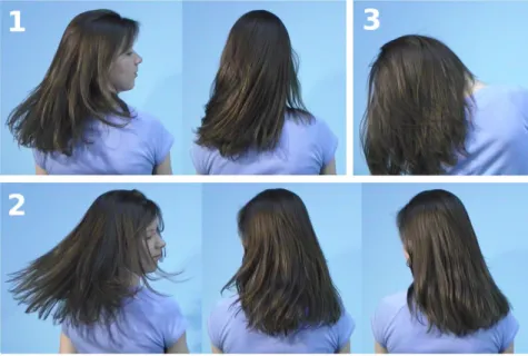
A human head of hair consists of about 150, 000 individual strands, which are very elon- gated, with a diameter of about 100µm for a potential length of dozens of centimeters. Con- versely, animal fur such as in Figure0.1(a)may contain millions of (generally shorter) strands.

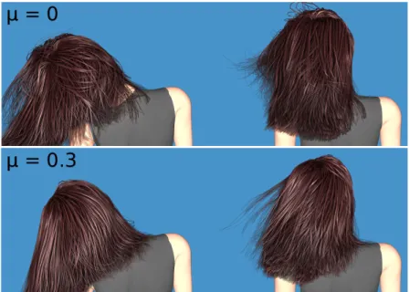
The relative importance of contact forces compared to other interactions, such as air drag or electostatic forces, is not well known. However, it is a certainty that contacts and friction play a huge role in the appearance of hair and fur, and proper handling of these interactions is of utmost importance for Computer Graphics applications. Indeed, frictional contacts maintain the volume of the groom, and thus the silhouette of the virtual character. Dry friction is furthermore responsible for the persistence of intricate patterns at rest, and ignoring it can lead to an uncan- nily tidy appearance. Despite these considerations, the work that we will present in Chapter4 was among the first to attempt to properly capture dry friction in hair simulations.

0.1.3 Target applications

In this dissertation, we will not attempt to quantitatively reproduce the behavior of the simulated materials in tightly controlled settings. Instead, we will be interested in capturing the qualitative characteristics of their large-scale dynamics.

This choice is partly motivated by applications to Computer Graphics, which we will discuss in more details below. Independently of the peculiarities of this industry, we believe that convincing simulations should be based on sound physics; when possible, we will also attempt to capture in our simulations the macroscopic laws that are experimentally observed to govern the materials.

(a)Hair dynamics, Chapter4 (b)Granular pressure, Chapter6

(c)Dry granular flows, Chapter7 (d)Immersed avalanches, Chapter8 Figure 0.2: A few snapshots of simulations from this manuscript

Moreover, we will not solely focus on Computer Graphics; for instance, Chapters6and8, in which we will study only 2D model problems, have no direct graphical application, and might be of greater interest to the mechanical engineering community.

Computer Graphics As already mentioned, a significant part of this work will be focused on devising simulation methods that are viable for Computing Graphics. A peculiarity of this ap- plication is that it strives to capture the emerging features that are created by the motion of the individual constituents. Indeed, while some of these features may not significantly influence the macroscopic mechanical properties of the material, they largely contribute to the visual richness of the overall phenomenon and would be extremely tedious to animate by hand. This overar- ching goal can thus be quite different from that of the mechanical engineering communities, so the simulation approaches will also be evaluated using different criteria. We list below a few of the virtues that numerical methods targeted at Computer Graphics should meet.

• realism, but notaccuracy. While the human mind is good at pointing out things that “feel off”, it is a poor judge about whether a simulated is physically accurate or not, especially as part of a heavily stylized movie. As such, we want to be able to capture qualitative features of our complex materials (for instance, the distinct regimes of granulars), but do not necessarily want to solve our equations to a high precision.

• artifacts-free. The resulting simulations must be free of disturbing visual artifacts, such asflickering,popping,privileged directionsorcreeping. Proper modeling of dry friction is necessary to avoid this last pitfall, and care has to be taken for the underlying discretization never to be visible.

• controllability. While physical realism is a good thing, being pleasant to the client’s eye is a prime requirement for any Computer Graphics simulation. If a gravity-defying hair wisp is required to achieve the desired look, then the numerical method should be able to handle it. Here, we will not worry too much about this aspect. However, we will prefer models based on measurable physical parameters, and shall ensure that implementation details such as a “number of solver iterations” do not affect too much the simulated physics.

• computational efficiency. As providing a good set of control parameters is a hard problem (see also Sigal et al.2015), a trial-and-error process is often required for artists to ob-

(A)

(B)

x_A=x_B n

Figure 0.3: Two bodies(A)and(B)are in contact when two points of their respec- tive surfaces, x_Aand x_B, coalesce. The resulting contact normal,n, is arbitrarily defined to point towards A.

tain a satisfying look. To make this process less painful, the numerical method should be reasonably efficient, and simulations for most shots should be able to finish overnight.

0.2 Contacts and dry friction

Proper modeling of invidual constituents (for instance, in the case of fibrous materials, choosing an adequate mechanical model for individual fibers) is obviously of primary importance for computing the dynamics of any complex material. However, we will not discuss this topic in this dissertation, and will simply rely on existing models from the literature. We will instead focus on the modeling and simulation of contacts and dry friction inside the material. We provide below a brief introduction to these physical phenomena, and present the modeling choices that will underpin the remainder of this dissertation.

0.2.1 Impacts

We assume the distinct constituents of our complex material to be large enough that they can be considered to never overlap. Impacts happen when two previously disjoint objects come into contact; that is, when their (initially positive) relative distance drops to zero. Assuming sufficient smoothness of their boundaries, the two bodies will then share a normal direction along the contacting surfaces, and further relative motion of each pair of contacting points will be restricted to the half-space spanned by this normal. The simplest scenario, where two locally smooth and convex bodies(A)and(B)come into contact, is illustrated in Figure0.3. Letx_A(t) andx_B(t)denote the position over time, for each object, of the surface point that will take part in the contact. The gapfunction, h(t) := x_A(t)−x_B(t), gives the relative position of those contacting points. The condition that objects(A)and(B)should not overlap can be written as

〈h(t),n〉 ≥0, wherenis the normal to(B)atx_Band〈·,·〉denotes the usual scalar product. The two objects are in contact at instanttifh(t) =0; as long as this is the case, the normal relative velocity,u_N(t):=_dh

dt,n

, should remain positive. Note thatucan be discontinuous at the time of impact; however, following Moreau (1988), we will assume locally bounded variations of the relative velocityu, i.e., the existence of a left-limit u(t⁻)and a right-limitu(t⁺)at every instantt.

At the onset of contact, a finitely-elastic body will compress, storing potential energy in the process, then restitute this energy in a second phase. Note that the amount of restituted energy does not depend on the “hardness” of the material, but rather on its internal structure; if this amount is high enough, the objects may end up separating themselves. If the elastic body is very stiff, these compression and decompression phases may happen on a time scale which is much lower than that of the studied system dynamics (Cadoux2009, Section 1.1.1). In order to avoid having to explicitly simulate this fine time scale, one may simply model the impact as an instantaneous jump of the relative normal velocities; several models have been proposed for this purpose. The simplest of them, the empirical Newton impact law, simply states that the post-impact normal velocity should be opposed and proportional to the pre-impact one, with a

material-dependentrestitutioncoefficient. On our simple example, this means that u_N(t⁺_i) =

−ξu_N(t⁻_i)≥0,t_idenotes the time of impact and where 0≤ξ≤1 is the restitution coefficient.

Note that this naive law may yield incorrect results in the presence of simultaneous contacts, and for instance will fail to reproduce the alternation in the contact points of a rigid block rocking on the ground; see (Brogliato1999) for more discussion about impact laws.

In this work, we will focus on the simplest case of purely inelastic impacts — the energy will be instantaneously dissipated by the system. We shall thus enforce the post-impact normal velocity,u_N(t⁺_i), to always be null, and refer to (Cadoux2009, Section 1.1.5) and (Smith et al.

2012) for suggestions about how the numerical framework used throughout this dissertation may be adapted to handle Newton-like impacts.

Signorini conditions Physically, the inter-penetration of the two objects is prevented by the onset of a contact-force,r. In the absence of friction and cohesion, this force should be colinear to the contact normal, i.e., r = r_Nn with r_N ≥ 0. Now, suppose that the two objects are in contact at timet, i.e.,h_N(t) =0. We have already stated the following conditions:

1. The normal relative velocity should be positive as long as the points are in contact, i.e., h_N=0 =⇒ u_N≥0.

2. Iftis a time of impact, the post-impact normal velocity,u_N(t⁺), should vanish.

3. The normal contact force should be positive, and vanish whenh_N>0.

The Signorini conditions are constructed by considering each contact in isolation, or more precisely, by assuming that the shock due to an impact does not propagate to other contacts.

This is consistent with our choice of a purely inelastic impact law, which already forbids energy restitution. In the more general setting of a Newton impact law, this means that the pre-impact velocities are computed independently for each contact point, or again that the work of the normal contact force at already existing contacts should not be strictly positive, i.e.,u_N(t⁻) = 0 =⇒ u_N(t⁺)r_N(t⁺)≤0. Another characterization of this hypothesis is that iftis not a time of impact for the considered contact, then the contact force should locally be of bounded variations att, i.e., should possess both left and right limits. Note that this strategy is unable to correctly model the famous Newton craddle, as the impacted balls would be incorrectly predicted to stick together (see Smith et al.2012, Figure 3, bottom).

Combining this new implication with the three previous ones, we get that





u_N(t⁺)≥0

r_N(t⁺) =0 ifu_N(t⁺)>0 r_N(t⁺)≥0 ifu_N(t⁺) =0

(1)

which together are known as theSignoriniconditions. Remember however that these velocity- level conditions apply only when the objects are in contact at instantt, i.e., whenh_N(t) =0.

The Signorini conditions are more commonly written in a more compact manner, making the use of complementarity notation and dropping the time variable, as

0≤u_N⊥r_N≥0,

where theu_N⊥r_Nnotation means that the two variables should be orthogonal, i.e.,r_Nu_N=0.

0.2.2 Dry friction

The set of inequalities commonly referred to as the Coulomb friction law is actually the result of observations made by several authors and over the span of many centuries (Besson2007). The discovery of the proportionality between the maximal tangential friction force and the normal load, as well as the irrelevance of the apparent contact surface area, are attributed to Leonard de Vinci at the end of the fifteenth century, and independently to Guillaume Amontons two hundred years later. Leonhard Euler distinguishes thestatic(or sticking) regime, when there is

r n α ϕ

α

g

Figure 0.4: Euler observed that as long as the angleαof an inclined plane remains below the friction angleϕ = arctanµ_S, the ratio of the tangential to normal components of the contact forcer will remain belowµ_S, and the body (gray) cannot not slide.

no relative motion between the two objects, from the dynamic regime, when one object is sliding on top of the other. Euler also introduced the notationµ_S for the staticfriction coefficient, i.e., the maximum ratio between the tangential and normal components of the reaction force, and related this coefficient to the maximum angleϕat which a mass may rest on an inclined plane without sliding asµ_S=tanϕ(see Figure0.4).

In his famed manuscript,Théorie des machines simples: en ayant égard au frottement de leurs parties et à la roideur des cordages, Coulomb (1781) compiled the results of several experiments, validating previous theories and noting that in the dynamic regime, the friction coefficient was independent of the sliding velocity. He also observed that for most materials, the static friction coefficient,µ_S, was higher than the dynamic one,µ_D. Overall, Coulomb observed the relation- ship between the normal and tangential forces as obeying

kr_Tk ≤µ_Sr_N ifu_T=0 (static regime)

kr_Tk=µ_Dr_N ifu_T6=0 (dynamic regime), (2) where the·Tdenotes the tangential part of the reaction force and relative velocity vectors, e.g., r_T = r −r_Nn. Incidentally, the proportionality of friction to the applied load was initially postulated by Amontons to be the result of the upper object having to elevate itself above the fine-scale irregularities of the contact surface. However, investigations in the twentieth century showed that this relationship is actually caused by an increase of the microscopic-level contact area when a higher normal load is applied (Bowden and Tabor1950).

In this work, we will not distinguish between the static and dynamic friction coefficients.

Indeed, the main characteristics of Coulomb friction, such as the existence of a sliding threshold that depends on the applied normal load, can already be captured without making this distinc- tion, and we did not judge the gain in realism brought by the introduction of a distinct sliding friction coefficient worth the significant associated increase in mathematical complexity³. Tak- ing into account the fact that the tangential friction force must oppose the sliding velocity, we will thus consider the Coulomb friction law as defined by the disjunction (3),





kr_Tk ≤µr_N ifu_T =0

§ kr_Tk=µr_N

r_T=−αu_T,α∈R₊ ifu_T 6=0. (3) 0.2.3 Other friction laws

While our work will be focused on Coulomb friction, we mention below a few other friction laws that are worthy of interest.

3In discrete-time numerical algorithms, the friction coefficient can always be updated explicitly at each timestep depending on the status of each contact point.

µr_N

−µr_N u_T r_T

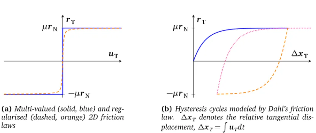
(a)Multi-valued (solid, blue) and reg- ularized (dashed, orange) 2D friction laws

−µr_N µr_N

∆x_T r_T

(b)Hysteresis cycles modeled by Dahl’s friction law. ∆xT denotes the relative tangential dis- placement,∆xT=R

u_Tdt

Figure 0.5:Some alternative friction laws: regularized (left) and Dahl’s (right)

Regularization In contrast to a fluid (orviscous) friction law, which could be defined as, say, r_T = −η(u)u_T, the Coulomb friction law (3) ismulti-valued. Foru =0, the friction force is not uniquely defined, but may lie anywhere inside a ball of radiusµr_N. As such, dealing with Coulomb friction will require devising specialized numerical method (Acary and Brogliato2008).

To avoid this complexity, one may choose toregularizethe law, writingr_T=−α(u_T,r_N)u_Twith, for instance,α(u_T,r_N):=min µr_N,¹_εku_Tk

/ku_Tk, orα(u_T,r_N):=µr_Nπ² arctan¹_εku_Tk /ku_Tk withεsmall, as in Figure0.5(a). However, such approaches may result in very stiff numerical systems, prone to flickering, and allow the lingering of creeping residual velocities; we will thus avoid this strategy.

Tresca model The Tresca friction law can be derived from the Coulomb law by removing the dependency of the friction force on the normal applied load,





kr_Tk ≤s ifu_T =0

§ kr_Tk=s

r_T=−αu_T,α∈R₊ ifu_T 6=0,

wheresis a positive scalar. As it reduces the coupling between tangential and normal compo- nents, the Tresca law is easier to handle numerically, yet still models a proper sliding thresh- old. However, the lack of proportionality of the frictional force to the applied load forbids the modeling of arbitrarily-sized stable heaps using Tresca friction, and we will thus discard this approximation.

Dahl model Taking inspiration from standard strain–stress diagrams, the Dahl (1968) fric- tion model describes the evolution of the friction force w.r.t. the relative tangential displace- ment, with a slope “reset” at each change of sign of the tangential velocityu_T. As depicted in Figure0.5(b), this model is able to capture hysteresis cycles induced by friction in loading–

unloading experiments, with a smooth reversing of the friction force, and has been especially popular to macroscopically account for the displacement of textile fibers under stretching and bending (Miguel et al.2013; Ngo Ngoc and Boivin2004). This smooth reversing of the friction force models slack in the sticking contact regime, and is therefore not really relevant for con- tacts between stiff bodies, which are close to slackless; we will thus not consider Dahl’s law in the following.

Rolling friction Rolling friction is induced by the deformation of a wheel near its contact point with the ground, and is responsible for energy dissipation that is not captured by the tangential Coulomb friction law (3). Indeed, Equation (3) implies that the work of the friction force is non-zero only when sliding occurs. However, in the remainder of this dissertation we will focus on stiff materials and relatively small applied loads, and will thus neglect rolling friction.

Figure 0.6: With Discrete Element Modeling, constituents are simulated individually, and all interactions between neighboring bodies must be taken into ac- count.

0.2.4 Discrete simulation of complex materials with frictional contacts

The most natural way to simulate complex materials numerically would be to follow the frame- work of Discrete Element Modeling (DEM),⁴that is, simulating individually each body and its interactions with the surrounding ones, as illustrated in Figure0.6.

As contacts and dry friction between the grains plays a primary role in the dynamics of com- plex materials, special attention should be given to the numerical treatment of those phenomena.

Different classes of approaches have been proposed in the literature, of which we can cite three:

• Molecular Dynamics(MD), which relax the assumption that distinct bodies cannot overlap, and use nonlinear springs to model the contacts between the particles (Cundall and Strack 1979). While this approach is the simplest to implement, limiting interpenetration can require the use of very stiff springs, which introduces a time scale much smaller than that of the macroscopic dynamics. This makes stable numerical integration difficult to achieve unless very small time steps are used, and may lead to visually disturbing flickering effects.

Moreover, how to handle multi-valued friction laws in the MD framework is not obvious, and as such creeping residual motion may plague this approach.

• Constraint-based approaches, such as theNon-Smooth Contact Dynamics(NSCD; Jean1999), propose to solve for each object’s dynamics while ensuring that the Signorini-Coulomb conditions (1) and (3) are satisfied. While being inherently more complex than MD, constraint-based approaches allow the use of larger timesteps, and thus still prove com- putationally efficient. Chapter 2will be dedicated to this kind of approaches, with an emphasis on the timestepping scheme proposed by Jean and Moreau (1987).

Scaling up The first part of this dissertation is dedicated to the simulation of dry frictional contacts in the DEM framework, using a constraint-based method; Chapter4presents results from the application of this strategy to hair dynamics. While those results were relatively good- looking, computational performance prevented us from simulating anything close to the whole 150, 000 individual fibers of a human head of hair. This motivated us to look for alternative approaches. Moreover, even though we were only simulating a small subset of the whole hair, we kept using afiber model for each simulated strand, while a wispmodel, representing the averaged behavior of several fibers, would have been more appropriate. Assuming the existence of such a model, we could as well take this approach one step further, and simulate the whole material using continuum mechanics.

As a first step towards the simulation of very large complex materials, the second part of this dissertation embraces this strategy, but focuses on simpler systems: granular materials consisting only of rigid grains. Devising a similar macroscopic simulation method for fibrous media such as hair remained out of the reach of this thesis.

4Note that the name DEM is also commonly used as a synonym for Molecular Dynamics; we use it here in a broader sense.

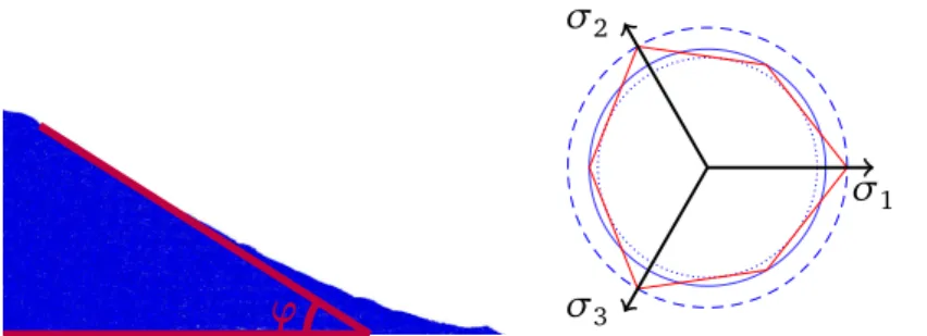
ϕ

σ

σ

σ

Figure 0.7: Left: visualization of the friction angleϕon a 2D granular heap at rest.

Right: 3D Mohr-Coulomb (red) with the three different Drucker-Prager yield surfaces (blue) in the plane of constant normal stressP

σ_i=3.

Using a continuum approach for granular materials makes sense, as they can beextremely large systems – a cubic meter of sand contains close to a trillion individual grains. We see imme- diately that simulating every grain as in the DEM framework, and taking into account each of its interactions with its neighbors, is not tractable, especially on standard computers. Moreover, the scale of inhomogeneities in granular materials is usually much smaller than the material itself.

For these reasons, several constitutive laws have already been proposed in the literature to model the macroscopic behavior of granulars. The next section introduces fundamental concepts for the continuum modeling of dry frictional contact in granular materials.

0.3 Continuum modeling of dry friction

When the discrete constituents are sufficiently small w.r.t. the scale at which a phenomenon is studied for the material to appear spatially homogeneous, averaging processes may be used to intuit constitutive equations (orrheologies) on macroscopic quantities such as stress and strain.

0.3.1 Yield-stress flows

For instance, the presence of large molecules in so-called Bingham plastics such as mayonnaise manifest itself at the macroscopic scale by the onset of ayield stressσ_S. This means that irre- versible deformations of the material will occur, i.e., the plastic strain rate ˙ǫwill be non-zero, only once the norm of the deviatoric stress,|Devσ|, has reached the critical valueσ_S. Such materials may remain indefinitely stuck in various shapes, in contrast to Newtonian fluids which will always, albeit potentially slowly, go back to a flat shape. Note that different choices can be used for the definition of the norm| · |in the above expression, yielding slightly different rhe- ologies, but anobjectivitycriterion should always be satisfied: one must ensure that the norm is invariant to changes in the reference frame. The Bingham model is classically defined us- ing the second invariant of the deviatoric part of the stress tensor,J₂(σ):= ¹₂Tr(Devσ)², with

|Devσ|:=p

J₂(σ). This definition ensures the objectivity of the model.

Such plastic phenomena are commonly described with a yield surface, that is, a function F, objective w.r.t. the stress tensor, such that the material remains solid whileF(σ)<0, and F(σ) =0 corresponds to the flowing regime where irreversible deformation occurs. The yield surface for the Bingham model is givenF^BI(σ):=p

J₂(σ)−σ_S. 0.3.2 Frictional yield surfaces

Granular materials also exhibit a yield stress, as demonstrated by their ability to form heaps that do not (systematically) collapse over time. However, just like Coulomb friction featured a sliding threshold proportional to the normal applied load, the yield stress of dry granular materials is observed to depend on the normal (ormean) stress, i.e., the internal pressure.

Mohr–Coulomb criterion The Mohr–Coulomb (MC) criterion is the continuum mechanics generalization of Euler’s inclined plane experiment, and consider the maximum angleϕ (the so-calledrest angle) that the slope of a granular heap can make without starting to avalanche (Figure0.7, left). Let us first consider the 2D case, and letσ_ϕ andτ_ϕ denote the normal and shear stresses acting on an inclined plane of angleϕ. By analogy with Euler’s criterion, the stability of the granular heap up to an angleϕmeans that the material’s yield condition can be writtenτ_ϕ≤σ_ϕtanϕ. Mohr’s circle relatesσ_ϕandτ_ϕ to the principal stresses of the material σ₁≤σ₂, i.e., the eigenvalues of theappliedstress tensor, as

σ_ϕ=−σ₁+σ₂

2 −σ₂−σ₁

2 sinϕ, τ_ϕ=σ₂−σ₁

2 cosϕ.

The cohesionless MC criterion thus states that a granular material with rest angleϕwill remain stable as long as

−σ₁+σ₂

2 −σ₂−σ₁ 2 sinϕ

tanϕ≥σ₂−σ₁ 2 cosϕ

−σ₁+σ₂

2 sinϕ≥σ₂−σ₁

2 . (4)

The 3D version of the Mohr-Coulomb criterion considers each plane of maximum shear, and can be summarized as

−σ₁+σ₃

2 sinϕ≥σ₃−σ₁

2 , (5)

whereσ₁ ≤ σ₂ ≤ σ₃ are the eigenvalues of the material’s stress. Inequation (5) written for each potential ordering of the eigenvalues defines 6 yield planes in principal stresses space; the MC yield surface is thus an hexagon-shaped convex cone centered around the hydrostatic axis σ₁ =σ₂= σ₃, as illustrated in Figure0.7, right. This hexagon degenerates to a triangle for sinϕ=1, and approaches a regular (yet vanishing) hexagon for sinϕ=0.

Note that while Coulomb friction is an approximation of interactions induced by the mi- croscopic asperities of the contacting surface between grains, Mohr–Coulomb theory averages grain-sized inhomogeneities, and is thus only valid at a much bigger scale.

Drucker–Prager yield criterion The Mohr–Coulomb criterion (5) involves the individual eigen- values of the stress tensor, and is numerically unwieldy. Drucker and Prager (1952) proposed a yield surface that is defined using only invariants of the stress tensor based on the Bingham model, but with a yield-stress that grows linearly with the first invariant of the stress tensor, I₁(σ):=Trσ. In the cohesionless case, the Drucker–Prager (DP) criterion is thus

Æ

J₂(σ) +µˆI₁(σ)

d ≤0, (6)

and ˆµis called the friction coefficient.

Note that in 2D, the Mohr–Coulomb and Drucker–Prager yield surfaces coincide. Indeed, I₁(σ) =σ₁+σ₂, andJ₂(σ) = ¹₄(σ₁−σ₂)²; Equations (6) and (4) thus become equivalent when ˆ

µ=tanϕ.

However, in 3D, direct computations yieldJ₂(σ) = ¹₆P

i6=j(σ_i−σ_j)²; the Drucker–Prager yield surface is thus a convex cone spanned by a circle centered on the hydrostatic axis (i.e., a Second-Order Cone). There is no hope for the DP and MC surfaces to fully match, but one may still choose the friction coefficient ˆµusing several heuristics (illustrated in Figure0.7, right):

• µˆ=²

p3 sinϕ

3−sinϕ , so that DP circumscribes MC;

• µˆ=^{q sinϕ}

1+¹₃sin²ϕ, so that DP inscribes MC;

• µˆ=²

p3 sinϕ

3+sinϕ , so that DP interpolates MC at middle vertices.

Choice between these different values is application-dependent. For instance, risk-assessment simulations may want to use the inscribed surface, so that the predicted run-out length of an avalanche with DP will always overestimate the one using MC.

Cohesion and tensile strength The Drucker–Prager model can be extended to the modeling of cohesive materials, modifying the yield surface as (Alejano and Bobet2012)

F_µ,ˆ^DP_ˆc(σ):=µˆI₁(σ)

d −ˆc+Æ

J₂(σ). (7)

A slightly more complex yield surface, the so-called Drucker–Prager yield surface withtension cut-off, may also be of interest for materials such as concrete. The cut-off dictates that the material will break when the mean tensile stress exceeds a critical valuecτ_c,

F_µ,ˆˆ^DP_c,cτ

c(σ):=max€

I₁(σ)−dcτ_c,F_µ,ˆˆ^DP_c(σ)Š

. (8)

The cut-off stress will influence the set of admissible stresses set only when there holds simul- taneouslyI₁(σ)≥ dcτ_c and ˆµI₁(σ)≤dˆc, which means ˆµcτ_c ≤ˆc; the original Drucker–Prager yield surface is retrieved when ˆµcτ_c≥ˆc. For this reason, we will prefer parameterizing the yield surface (9) with a shear yield stress,σ_S:=ˆc−µcˆτ_c, rather than with the cohesion coefficient ˆc.

In the following, we will thus write the Drucker–Prager yield surface with tension cut-off as F_µ,σˆ^DP

S,cτ_c(σ):=max



I₁(σ)−dcτ_c, ˆµI₁(σ)−dcτ_c

d −σ_S+Æ J₂(σ)

‹

. (9)

Note that the Bingham yield surface is recovered whencτ_c= +∞.

Other yield surfaces Both the Mohr–Coulomb and Drucker–Prager yield surfaces are nons- mooth; the normal to the surface is not uniquely defined everywhere, in particular forσ=0 in the cohesionless case. As we will see in Chapter1, this complicates the definition of a flow rule, that is, we will not be able to unambiguously express the direction of plastic displacement as a function of the stress tensor. ‘ Mast (2013) presents different strategies to circumvent this difficulty, such as using a smooth cap for the Drucker–Prager cone, or prescribing the flow to be along the hydrostatic axis whenσ=0. Another interesting option that they explore is the use of the Matzuo–Nakai yield surface, which is smooth everywhere and better matches the hexagonal shape of the Mohr–Coulomb surface that the Drucker–Prager law.

0.3.3 Shearing granular flows

The “GDR MiDi” group (GDR MiDi2004) studied dense granular shearing flows, and proposed a new constitutive law that was able to match experiments quantitatively, the so-calledµ(I) rheology (Jop et al.2006). Based on the Drucker–Prager yield criterion, this rheology suggests to vary the friction coefficient with theinertial number I,

I(˙ǫ,σ):=

pJ₂(˙ǫ)D_g ÆI₁(σ)/(dρ_g),

where ˙ǫis the strain rate,D_gthe average diameter of grains, andρ_gtheir density. This dimen- sionless number relates the fluctuation of the velocity at the grain scale to that of the macroscopic flow. WhenI =0, the material behaves like a solid, and for very high values ofI, the material becomes akin to a gas; in between lies the dense flowing regime.

Shear-hardening friction The higher the inertial number, the more energy will be dissipated by grain–grain interactions, and the higher the friction coefficient should be. Jop et al. (2006) propose the following expression:

µ(I) =µ_S+µ_D−µ_S I₀/I+1,

withµ_D ≥µ_S and where I₀ is a material-dependent constant. In contrast to discrete friction laws which are usually taken to be slip-weakening (e.g., Coulomb friction whenµ_S> µ_D), the µ(I)rheology is thus shear-hardening.

Note that theµ(I)rheology does not influence the rest angle of the material; at rest,I =0 andµ(I) =µ_S.

Dilatancy In a similar manner, the volume fraction of grainsφ, that is, the fraction of space occupied by the granular material, can be affected by the shear rate; when this translates into an augmentation of the flow volume, this phenomenon is known asdilatancy. In dense shearing flow, the volume fraction has been observed to decrease with the inertial number (GDR MiDi 2004). Roux and Radjai (1998) define the dilatancy angleψfrom the ratio between the volu- metric and shear strain rates, ¹_dI₁(˙ǫ)tanψ=J₂(˙ǫ). They relate this angle to a critical volume fractionφ_c asψ(φ) =ψ₀(φ−φ_c), so that positive dilatancy occurs above the critical volume fraction, but shear tends to compress the material whenφ < φ_max.

0.3.4 Other complex materials

This section has made clear that devising macroscopic laws for granular materials, even when assuming perfectly rigid and spherical grains, was already complex. Continuum modeling of as- semblies of elastic and anisotropic objects such as fibers would require much more sophisticated models, and was thus left out of the scope of this dissertation.

0.4 Synopsis

This dissertation will be divided in two parts. The first one wi