Modélisation à base de réseaux de neurones dédiés à la prédiction sous incertitudes appliqué aux systèmes

Les prévisions de demande et de production énergétique peuvent être intégrées directement dans la gestion opérationnelle des unités. Cet objectif est atteint à travers deux méthodes d’estimation des IP de vitesse du vent à court terme dans le cadre d’une nouvelle approche de l’ensemble des NN.

Figure 1. La structure le MLP utilisée dans cette thèse pour construire les PIs.

INTRODUCTION

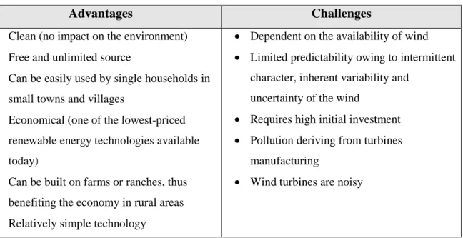
Energy Sector: issues, challenges and needs
The Adequacy Assessment of Distributed Power Generation Systems
The Prediction Problem and Its Role in the Adequacy Assessment of Distributed Power Generation Systems
The Research Problem and Motivation

8 Prediction intervals (PIs) are a simple way of communicating a measure of the uncertainty in the predictions. Visualization of the flow (motivation, focus and methods) of the thesis work on the forecasting problem in the context of adequacy assessment of wind integrated distributed generation systems.

Figure 1. Total primary energy supply by source (source: World Energy Resources Survey 2013) [1]

THE PREDICTION PROBLEM 1 Problem Statement

Methods .1 Regressions

Machine learning methods
Methods for wind speed/power and load forecasting

Over the years, several stationary and non-stationary models have been developed and used in the literature for time series forecasting. Some works exist that use meteorological variables (e.g. temperature, humidity, cloud cover, etc.) to predict the load, while others treat the load pattern as a time series signal and predict the future load using various time series analysis techniques. [62].

PIs Definition

These methods that only provide point predictions cannot properly handle both the uncertainty in the model parameters and the noise in the input data. Although the point forecasts are relatively easy to calculate and easy to understand, the main motivation for constructing PIs is to quantify the associated uncertainty in the point forecasts.

Figure 3. Exemplification of the terminology and concept of a prediction interval [45]

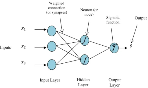
ARTIFICIAL NEURAL NETWORKS (NNs) FOR PREDICTION 1 Basics of NNs modeling

Training of NNs

The values of the weight vector w characterizing the network are thus optimized during training. The implementation details of the back-propagation algorithm and its mathematical formulation can be found in.

Over-fitting and Cross-validation

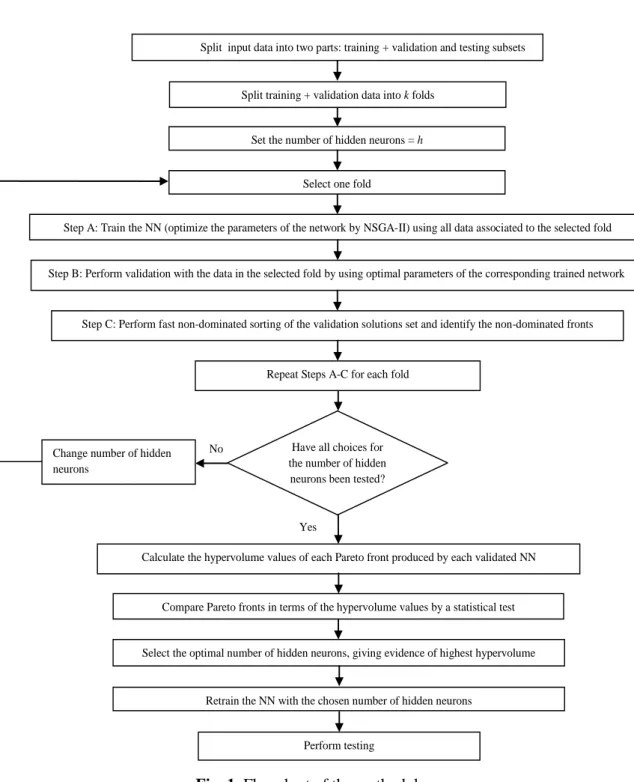
It is also used for model selection [87] and for determining the optimal network architecture (i.e., the number of hidden neurons) [88]. In this line of research, in Paper I of Part II, a systematic process has been followed to identify the optimal NN structure (i.e. the number of hidden neurons) via CV.

PIs Estimation by NNs

The common feature of the PI estimation methods mentioned above is that they do not consider the width of the intervals in the estimation process [35]. Note that the approach proposed in this research work integrates PI estimation into its learning procedure, while other methods except LUBE construct PI in two steps (first making point prediction and then constructing PI).

Figure 7. Architecture of a MLP NN model for estimating the lower and upper bounds of PIs

Single-objective Optimization: Genetic Algorithms and Simulated Annealing A single-objective optimization problem (SOP) involves a single objective (cost) function and

Mutation is the change of the value of each bit of a chromosome with a certain probability (namely the mutation probability or mutation rate). A schematic of the standard procedure for a basic GA for a maximization problem is given in Figure 8.

Multi-objective Optimization: Non-dominated Sorting Genetic Algorithm-II (NSGA-II)

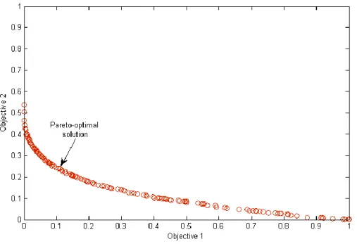
Thus, a Pareto optimal set is a set of solutions that are not dominated with respect to each other when all objectives are considered. The solutions that are not dominated within the entire search space are referred to as Pareto optimal and form the Pareto optimal set; the corresponding values of the objective functions form the so-called Pareto-optimal front in the objective function space (see Figure 10). The Pareto-optimal set of solutions can provide the DMs with the flexibility to select appropriate solutions, balancing different preferences against the objectives.

Training of NNs by NSGA-II

For each input sample in the training set, estimate each of the chromosomes in the initial population, i.e. calculate the lower and upper bounds of the outputs of each chromosome with the parameters by performing NN training. 41 In the end, the best front is selected based on the ranking of non-dominance and diversity of individual solutions. Thus, according to the original NSGA-II definition, we performed binary tournament selection, mutation and crossover in the initialization phase.

APPLICATIONS

Prediction of Scale Deposition Rate in Oil & Gas Equipment

We here use a systematic approach, rather than a trial and error method, for choosing the optimal number of hidden neurons in the hidden layer. For comparison purposes, we have also calculated the CWC values of the optimal Pareto front solutions extracted by MOGA for the training and test sets. The MOGA-NN approach integrates PI estimation into the learning procedure of the algorithm.

Table 4. Descriptive Statistics of CPU times (s) of twenty MOGA, SOSA and SOGA on winter training dataset

UNCERTAINTY TREATMENT: INTERVAL-BASED ESTIMATED PREDICTION INTERVALS

Problem Statement

Interval Analysis

Our adequacy assessment framework leads to the estimation of EENS based on interval-evaluated load and wind energy input data. Similarly, the central values (midpoint) of the PI were used as input values to estimate the ENS mean. In contrast, training NN with historical wind speed data ensures that the time dependence between successive observations is taken into account, leading to more accurate predictions.

UNCERTAINTY TREATMENT: NN ENSEMBLES 1 Construction of an Ensemble of NNs

Application to Wind Power Prediction Intervals Estimation with Interval Wind Speed Inputs

The inherent stochasticity in the power curve is motivated by the fact that different wind turbines correspond to specific power curve parameters, leading to an inaccurate and imperfect knowledge of the power curve transformation. In this way, epistemic uncertainty resulting from the imperfect knowledge of the power curve parameters is also taken into account by means of bootstrap sampling. The invariance of the coverage probability by going from wind speed to wind power PIs was also shown.

Application to Short-term Wind Speed Prediction Intervals Estimation

The user-specified parameters of NN and NSGA-II, and the plots of the resulting mean bootstrapped PIs for 1-h wind power prediction are given in the paper. Compared to literature methods that are conceptually and methodologically similar to the present ones, the obtained results show a significant improvement in terms of the quality of the predicted PIs. We can therefore conclude that both proposed ensemble modeling frameworks provide a reliable estimation of the PIs, characterized by a high coverage probability and a small interval size.

CONCLUSIONS

Methodological and applicative contributions

In the phase of combining selected individual NN results, we used a k-nn approach to identify similar patterns between training and test sets. 64 It should be emphasized that solving the regression problem also requires adequate preliminary processing of the input data. For time series forecasting, the number of prior lags associated with the outcome is also a key factor to get right.

Future Work

Zio, "An Interval-Valued Neural Network Approach for Prediction Uncertainty Quantification", IEEE Transactions on Neural Networks and Learning Systems, 2014, (under review). Khosravi, “Short-term load and wind power forecasting using neural network-based prediction intervals”, IEEE Transactions on Neural Networks and Learning Systems, vol. Nahavandi, "Combined Nonparametric Prediction Intervals for Wind Power Generation", IEEE Transactions on Sustainable Energy, vol.

NSGA-II-trained neural network approach to the estimation of prediction intervals of scale deposition rate in oil & gas equipment

NSGA-II Trained Neural Network Approach for Estimation of Scale Deposition Rate Prediction Intervals in Oil and Gas Equipment. NSGA-II Trained Neural Network Approach for Estimation of Scale Deposition Rate Prediction Intervals in Oil and Gas Equipment.

NSGA-II-Trained Neural Network Approach to the Estimation of Prediction Intervals of Scale Deposition Rate in Oil & Gas Equipment

MODELING FRAMEWORK

NSGA-II optimization of a NN for PIs estimation

82 optimal set, the corresponding values of the objective functions form the so-called Pareto optimal front in the objective functions space. NSGA-II is one of the most efficient multi-objective evolutionary algorithms (Deb, Agrawal, Pratap, & Meyarivan, 2002). Finally, the best front in terms of ranking of non-dominance and diversity of the individual solutions is selected.

MODEL IDENTIFICATION

Comparison of Pareto fronts by the hypervolume indicator

Boxplots of the total hypervolume scores for different numbers of hidden neurons with respect to the training dataset. Boxplots of the total hypervolume scores for different numbers of hidden neurons with respect to the validation dataset. The hypervolume values of the Pareto fronts produced after retraining the NN with different numbers of hidden neurons.

CONCLUSION AND FUTURE WORK

In Proceedings of the 10th International Flins Conference on Uncertainty Modeling in Knowledge Engineering and Decision Making (Flins 2012), Istanbul, Turkey. In Proceedings of the Tenth ACM SIGEVO Workshop on Foundations of Genetic Algorithms (Foga'09) (pp Orlando, USA. In Proceedings of the International Conference on Theory and Applications of Mathematics and Informatics (ICTAMI 2004), Thessaloniki, Greece.

Multi-objective Genetic Algorithm Optimization of a Neural Network for Estimating Wind Speed Prediction Intervals

NNS AND PIS

Two measures are used to evaluate the quality of PI: coverage probability (CP) and interval width (IW) [11-13]. 2014), submitted to Applied Soft Computing (under review).. 104 of the objectives and to improve the generalization performance of the model [11]. The function ( ) is equal to 1 during training, while in NN testing it is given by the following step function:. 2014), submitted to Applied Soft Computing (under review).

MULTI-OBJECTIVE OPTIMIZATION BY NSGA-II

Solutions that are not dominant in the entire search space are labeled as Pareto-optimal and constitute the Pareto-optimal set; the corresponding values of the objective functions form a so-called Pareto-optimal front in the space of the objective functions. Decision makers also gain insight into the characteristics of the optimization problem before making a final decision. We resort to GA to set the NN weight values for PI estimation.

Mutation involves changing the value of each gene in a solution with a predefined probability (the mutation rate) [39]. The overall computational complexity of the proposed algorithm can be explained in terms of two time-consuming sub-operations: non-dominated sorting and fitness evaluation. The time complexity of the non-dominated sorting part is ( ), where is the number of targets and is the population size [14].

EXPERIMENTS AND RESULTS

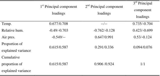
Pre-Treatment of Input Data
NN Training and Testing Results
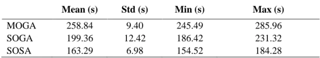
MOGA comparison with SOSA and SOGA
Comparison with MO-CMA-ES

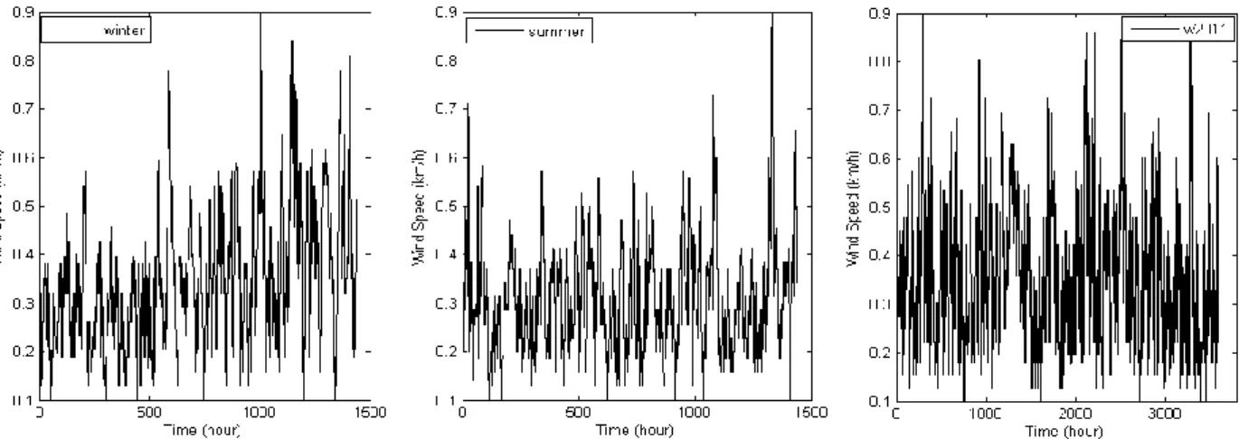
The final choice regarding model input for the NN model is the number of past wind speed values to consider. The overall best Pareto front obtained by training NN for 1-h-ahead wind speed prediction: winter period (left) and w2011 period (right). 13 shows the convergence behavior of PICP and NMPIW through the iterations of MOGA for the winter dataset.

Fig. 5, top, left for winter and right for summer) shows a non-negligible correlation of the wind speed time series, also for high values of the lag

Two Machine Learning Approaches for Short-Term Wind Speed Time Series Prediction

BASICS OF THE TWO MACHINE LEARNING APPROACHES 1. Prediction Intervals

Quantifying the Prediction Intervals by Multi-Layer Perceptron Neural Networks Trained by MOGA
Quantifying the Prediction Intervals with ELM Regression and the Nearest Neighbors Approach
General Concepts of Extreme Learning Machines

In the final step, the performance of the estimated prediction intervals can be assessed by calculating the coverage probability (PICP) and the widths of the prediction intervals (PIW). Determine for each of the patterns in the test data set the nearest neighbors from the training data set. Sort the nearest neighbor errors for each of the patterns in the test data set.

CASE STUDY AND RESULTS 1. Applied Datasets

Pre-analysis of input data for MOGA MLP NN
Prediction Results with ELM and Nearest Neighbors Approach

The choice of the number of lagged time series inputs for the ELM algorithm can be directly based on considerations relevant to PI estimation. Due to the computational efficiency of ELM, the computation times for training and also for testing are negligible. To evaluate the performance of the proposed approach for evaluating PI in testing.

Fig. 2. The wind speed datasets used in this study: winter (left), summer (middle) and w2011 (right)

Discussion of the strengths and limitations of the selected approaches

The 152 datasets, PICP and NMPIW are created in a similar way to evaluate the performance of the MOGA NN approach. This characteristic of the data set imposed limitations on the flexibility and accuracy of the applied approach. Moreover, the errors of the training data set can be weighted, according to the distance of the models in the input space.

CONCLUSION

Atiya, “A comprehensive review of neural network-based prediction intervals and new developments,” IEEE Transactions on Neural Networks, vol. Atiya, “A Lower Upper Bound Estimation Method for Neural Network-Based Prediction Interval Construction,” IEEE Transactions on Neural Networks, vol. Huang, “Learning capacity and storage capacity of two-layer feed-forward networks,” IEEE Transactions on Neural Networks, vol.

An Interval-Valued Neural Network Approach for Prediction Uncertainty Quantification

NEURAL NETWORKS AND PREDICTION INTERVALS

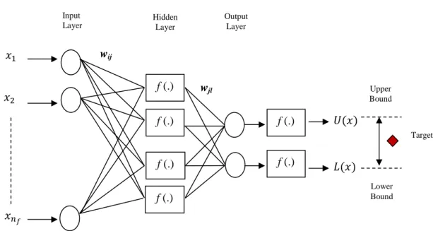
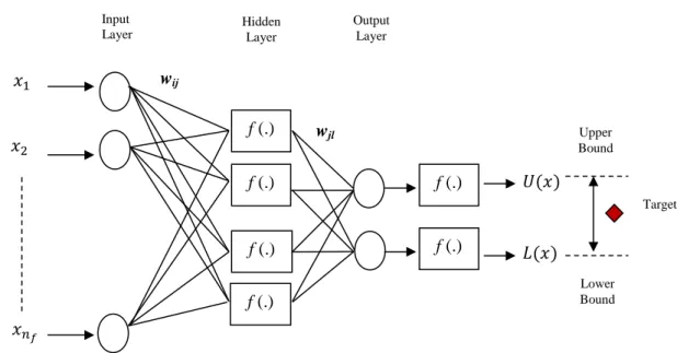
It is common to think of a NN model as a way to solve a nonlinear regression problem. To evaluate the quality of the PIs, we take the prediction interval coverage probability (PICP) and the prediction interval width (PIW) as measures: the former represents the probability that the set of estimated PIs will contain the true output values ( ) (must be maximized), and the latter simply measures the extension of the interval as the difference between the estimated upper limit and lower limit values (to be minimized). When interval-valued data [24] is used as input, each input pattern is represented as an interval, where are the lower and upper limits, respectively (real values ) of the input interval.