Modelling constraints on the emission inventory and on vertical diffusion for CO and SO2 in the Mexico City Metropolitan Area using Solar FTIR and zenith sky UV

(1)

HAL Id: hal-00303940

https://hal.archives-ouvertes.fr/hal-00303940

Submitted on 11 Jul 2006

HAL is a multi-disciplinary open access archive for the deposit and dissemination of scientific research documents, whether they are published or not. The documents may come from teaching and research institutions in France or abroad, or from public or private research centers.

L’archive ouverte pluridisciplinaire HAL, est destinée au dépôt et à la diffusion de documents scientifiques de niveau recherche, publiés ou non, émanant des établissements d’enseignement et de recherche français ou étrangers, des laboratoires publics ou privés.

Modelling constraints on the emission inventory and on vertical diffusion for CO and SO2 in the Mexico City Metropolitan Area using Solar FTIR and zenith sky UV

spectroscopy

B. de Foy, W. Lei, M. Zavala, R. Volkamer, J. Samuelsson, J. Mellqvist, B.

Galle, A.-P. Martínez, M. Grutter, L. T. Molina

To cite this version:

B. de Foy, W. Lei, M. Zavala, R. Volkamer, J. Samuelsson, et al.. Modelling constraints on the emission inventory and on vertical diffusion for CO and SO2 in the Mexico City Metropolitan Area using Solar FTIR and zenith sky UV spectroscopy. Atmospheric Chemistry and Physics Discussions, European Geosciences Union, 2006, 6 (4), pp.6125-6181. �hal-00303940�

(2)

ACPD

6, 6125–6181, 2006

Sources and transport of CO and

SO₂ in the MCMA B. de Foy et al.

Title Page Abstract Introduction Conclusions References

Tables Figures

J I

Back Close

Full Screen / Esc

Printer-friendly Version Interactive Discussion

EGU Atmos. Chem. Phys. Discuss., 6, 6125–6181, 2006

www.atmos-chem-phys-discuss.net/6/6125/2006/

Atmospheric Chemistry and Physics Discussions

Modelling constraints on the emission inventory and on vertical di ff usion for CO and SO ₂ in the Mexico City Metropolitan Area using Solar FTIR and zenith sky UV spectroscopy

B. de Foy¹, W. Lei², M. Zavala², R. Volkamer³, J. Samuelsson⁴, J. Mellqvist⁴, B. Galle⁴, A.-P. Mart´ınez⁵, M. Grutter⁶, and L. T. Molina^1,2

1Molina Center for Energy and the Environment, CA, USA

2Department of Earth, Atmospheric and Planetary Sciences, Massachusetts Institute of Technology, USA

3Department of Chemistry and Biochemistry, University of California, San Diego, USA

4Department of Radio and Space Science, Chalmers University of Technology, Gothenburg, Sweden

5General Direction of the National Center for Environmental Research and Training (CENICA), National Institute of Ecology (INE), Mexico

6Centro de Ciencias de la Atm ósfera, Universidad Nacional Aut ónoma de M éxico, M éxico Received: 19 June 2006 – Accepted: 20 June 2006 – Published: 11 July 2006

Correspondence to: B. de Foy ([email protected])

(3)

ACPD

6, 6125–6181, 2006

Tables Figures

J I

Back Close

Full Screen / Esc

EGU Abstract

Emissions of air pollutants in and around urban areas lead to negative health impacts on the population. To estimate these impacts, it is important to know the sources and transport mechanisms of the pollutants accurately. Mexico City has a large urban fleet in a topographically constrained basin leading to high levels of carbon monoxide (CO).

5

Large point sources of sulfur dioxide (SO₂) surrounding the basin lead to episodes with high concentrations. An Eulerian grid model (CAMx) and a particle trajectory model (FLEXPART) are used to evaluate the estimates of CO and SO₂in the current emission inventory using mesoscale meteorological simulations from MM5. Vertical column measurements of CO are used to constrain the total amount of emitted CO in

10

the model and to identify the most appropriate vertical diffusion scheme. Zenith sky UV spectroscopy is used to estimate the emissions of SO₂ from a large power plant and the Popocat ´epetl volcano. Results suggest that the models are able to identify correctly large point sources and that both the power plant and the volcano impact the MCMA. Modelled concentrations of CO based on the current emission inventory

15

match observations suggesting that the current total emissions estimate is correct.

Possible adjustments to the spatial and temporal distribution can be inferred from model results. Accurate source and dispersion modelling provides feedback for development of the emission inventory, verification of transport processes in air quality models and guidance for policy decisions.

20

1 Introduction

Detailed and accurate emission inventories are a cornerstone of effective air quality management programs. Public policy choices can be evaluated with air quality models based on actual emissions and alternative scenarios in combination with accurate meteorological simulations. This paper makes use of novel measurement techniques

25

to evaluate the carbon monoxide (CO) inventory for the Mexico City Metropolitan Area

(4)

ACPD

6, 6125–6181, 2006

Tables Figures

J I

Back Close

Full Screen / Esc

EGU (MCMA) and to evaluate the potential impacts of large point sources of sulfur dioxide

(SO₂). Even though vertical diffusion has a large impact on pollutant transport, it can be overlooked as a source of uncertainty. Pollution observations and simulations are further used to evaluate alternative vertical diffusion schemes.

1.1 Mexico City Metropolitan Area

5

Megacities are home to a growing number of people and can suffer from high levels of air pollution (Molina and Molina,2004;Molina et al.,2004). The MCMA is a megacity of around 20 million people living in a basin 100 km diameter. The basin is surrounded by high mountains on the west, south and east and is located at high elevation, leading to intense solar radiation and high ozone levels most of the year. There has been

10

extensive scientific study of the air quality in the MCMA, as reviewed inMolina and Molina (2002).

Nickerson et al.(1992) carried out aircraft profiles of ozone, SO₂and particulate matter (PM) above Mexico City in 1991, highlighting the importance of combustion sources for the basin air pollution. Williams et al. (1995) modelled air dispersion for the same

15

episodes looking at the transport of contaminants towards the southwest of the basin and emphasizing the need for improved accuracy of the emission inventory.Elliott et al.

(1997) analyse the importance of liquefied petroleum gas (LPG) components in the urban air chemistry. By estimating CO life times of approximately 2 days in the basin, estimates are made of the LPG venting to the regional environment.

20

Fast and Zhong(1998) developed a wind circulation model for the basin from data obtained during the IMADA campaign of 1997. This emphasized the importance of vertical mixing and mountain winds in the transport of the urban plume first towards the south and then back over the city to the north. Similar patterns are described in Jazcilevich et al.(2003) with evidence of direct convective transport from layers aloft

25

to the surface. West et al.(2004) modelled the photochemistry in the basin during the IMADA campaign, suggesting that the emission inventory for CO be scaled by a factor of 2 and that of volatile organic compounds (VOCs) by a factor of 3.

(5)

ACPD

6, 6125–6181, 2006

Tables Figures

J I

Back Close

Full Screen / Esc

EGU MCMA-2003 was a major field campaign that took place in April 2003.De Foy et al.

(2005) classified the meteorological conditions into 3 episode types which were sub- sequently used to analyse the transport and basin venting (de Foy et al., 2006c). In particular, this found short residence times in the basin and little carry-over from day to day.

5

1.2 Emission inventory

Emission inventories can be derived using either the “top-down” method, where total fuel and energy consumption are used for a whole region to determine surface emissions or the “bottom-up” method, where estimates of vehicle miles travelled and residential, industrial and commercial energy use patterns are considered. The 2002

10

official emission inventory for the MCMA used in this study was derived by the bottom- up method by the Comisi ´on Ambiental Metropolitana (CAM) of the Mexican Federal District government (Comisi ´on Ambiental Metropolitana, 2004). This contains annual totals for the criteria pollutants which need to be temporally and spatially distributed as well as speciated for VOCs (West et al.,2004).

15

Schifter et al. (2005) develop a top-down estimate of vehicular emissions by combining fuel use statistics with emission factors obtained from in-situ remote sensing experiments. This suggests that there has been a reduction in MCMA emissions and that, if anything, the official inventory may overestimate CO emissions. Jiang et al.

(2005) obtain emission factors for the MCMA vehicle fleet by analysing data from the

20

Aerodyne mobile laboratory (Kolb et al., 2004) for CO, black carbon, polycyclic aro- matic hydrocarbons and other pollutants. For CO, a similar conclusion toSchifter et al.

(2005) is drawn, that official inventory estimates are high but in general agreement.

Zavala et al.(2006) analyse chase and fleet average mode data in detail, determining emission factors from individual vehicle plumes and obtaining emission estimates for

25

individual vehicle types. This provides valuable information on NO_x, aldehydes, ammo- nia and certain VOC’s which will be used to further refine the emission inventory and guide policy work.

(6)

ACPD

6, 6125–6181, 2006

Tables Figures

J I

Back Close

Full Screen / Esc

EGU On a more regional scale, Kuhns et al. (2005) report on the development of an

emission inventory for the northern part of Mexico as part of the BRAVO study. This includes the MCMA inventory but not the surrounding region. Olivier and Berdowski (2001) develop the EDGAR global emission inventory at a 1 degree resolution. For Mexico however, the MCMA is about ten times larger than anthropogenic sources out-

5

side of the basin. This means that within the accuracy of the present modelling work, regional emissions can be represented through appropriate settings of the boundary conditions.

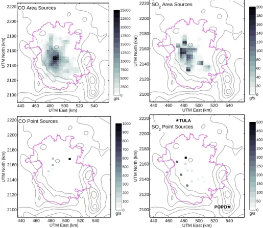
The BRAVO emission inventory also includes estimates of SO₂ emissions from the Popocat ´epetl volcano and the Tula industrial complex, two large point sources shown in

10

Fig.1. The Tula source consists of both a power plant and a refinery. The Popocat ´epetl volcano is an active volcano forming the south-eastern edge of the MCMA basin. It has been under continuous monitoring by the Centro Nacional de Prevenc´ıon de Desastres (CENAPRED).Kuhns et al.(2005) report SO₂emission estimates made with a correlation spectrometer (COSPEC) as high as 50 000 tons/day (metric) but more typically

15

around 3000 to 5000 tons/day. Galindo et al. (1998) analyse the gas and particle emissions during the eruptions of December 1994 to January 1995. They report a baseline SO₂ emission rate of 1000 tons/day rising up to 5000 tons/day during eruptions. Delgado-Granados et al. (2001) further analyse COSPEC data to distinguish between pre-eruptive emissions of 2000 to 3000 tons/day and effusive-explosive pe-

20

riods with emissions up to 13 000 tons/day. They therefore classify the volcano as a high-emission rate, passively degassing eruptive volcano. This means that high SO₂ emissions are present in the absence of any visible ash plume. Wright et al. (2002) make use of GOES satellite thermal imagery to identify explosions, exhalations and cycles of dome growth of the volcano, which can be indicative of increased SO₂emis-

25

sions. Matiella et al. (2006)¹ use MODIS data to quantify the size of ash and SO₂

1Matiella, M. A., Watson, I. M., Delgado-Granados, H., Rose, W. I., and Cardenas-Gonzalez, L.: Volcanic emissions from Popocatepetl volcano, Mexico, quantified using Moderate Resolu- tion Imaging Spectroradiometer infrared data, J. Volcanol. Geotherm. Res., in review, 2006.

(7)

ACPD

6, 6125–6181, 2006

Tables Figures

J I

Back Close

Full Screen / Esc

EGU clouds. SO₂ emission rates were found in broad agreement with COSPEC values of

5000 to 32 000 tons/day.

Regional export of sulfate aerosols was simulated byBarth and Church(1999) with a global model along with black carbon transport and oxidation. Mexico City was found to contribute approximately 1% to the global sulfate burden. Marquez et al. (2005)

5

measured air quality 250 km east of the MCMA near a mountain top to further evaluate the effects of urban emissions on the regional environment. Volcanic degassing of SO₂ was not considered as a possible additional source however (Pyle and Mather,2005).

Raga et al.(1999) had previously analysed SO₂, CO and aerosol measurements in the MCMA and suggested that increased sulfate aerosol production in the city could

10

be due to volcanic emissions. Jimenez et al.(2004) report on a field study carried out between Popocat ´epetl and Puebla (to the east). Clear evidence was found of volcanic influence at the surface for 6 out of 17 days sampled.

1.3 Measurements

Column measurements of CO can be used in conjunction with dispersion models to

15

constrain emission inventories. For example,Yurganov et al.(2004) obtain CO columns from Fourier Transform Infrared (FTIR) spectrometers. A box model and the 3-D global GEOS-CHEM model (Bey et al.,2001) are used to evaluate the emissions from boreal wild fires in August 1998. Yurganov et al. (2005) extend the analysis to 2002 and 2003. Strong correlations are found between estimates from surface measurements

20

and those from MOPITT CO columns.

Remote sensing of SO₂ can be used to estimate emission rates. Whereas CO sources are spread out and CO plumes broad, SO₂ sources are more likely to be large point sources with individual well-defined plumes. Galle et al. (2003) develop a miniaturised ultraviolet sprectrometer to evaluate volcanic emissions. The “Mini-DOAS”

25

is used to quantify emissions from 2 volcanoes and is compared with measurements from COSPEC.Elias et al.(2006) report further validation against COSPEC with agreement between the different systems within 10%. McGonigle et al.(2004) use the same

(8)

ACPD

6, 6125–6181, 2006

Tables Figures

J I

Back Close

Full Screen / Esc

EGU technique for estimating power plant emissions of both SO₂and NO₂. Emission rates

of 5.2 kg/s of SO₂were remarkably close to in-stack monitor values of 5.3 kg/s, suggesting that this method provides an accurate, low-cost, easily deployable means of estimating and validating large point sources in emission inventories.

1.4 Source identification

5

Blanchard (1999) reviews different methods for estimating the impacts of emission sources on air pollutant levels. These can be separated into data analysis methods and model-based methods. The latter includes forward and backward trajectory analyses as well as Eulerian dispersion models.Hopke(2003) reviews further developments of receptor models and back trajectory analyses. “Residence Time Analysis” and “Po-

10

tential Source Contribution Function” are described and compared using case studies in the northeast of the U.S.

“Residence Time Analysis” was introduced by Ashbaugh et al. (1985). It is a 2-D gridded field that represents the probability that a randomly selected air parcel is to be found in a grid cell relative to the total time interval of the trajectory. Dividing the

15

probability of a “dirty” air parcel being in a grid cell with the probability of any air parcel passing through that cell, one obtains the “Potential Source Contribution Function”.

This normalised field will have high values over regions of high emissions. The method was used to show that the dominant source of sulfur in the Grand Canyon national park was from southern California.

20

Sirois and Bottenheim(1995) define “Probability of Residence” by applying the Res- idence Time Analysis ofAshbaugh et al.(1985) to the trajectories associated with the highest and lowest 10% of air pollutant concentrations. A cluster analysis was then performed on all backward trajectories at the receptor site. Analysis of the pollution levels associated with each cluster showed agreement with the “Probability of Residence”

25

method while providing additional information about air mass movements. Vasconce- los et al. (1996a) apply the method of Ashbaugh et al.(1985) to field campaign data in the Grand Canyon, again identifying southern California as the main source region.

(9)

ACPD

6, 6125–6181, 2006

Tables Figures

J I

Back Close

Full Screen / Esc

EGU The spatial resolution of their results is analysed inVasconcelos et al. (1996b). This

suggested that the method has good resolution in source direction but significantly less in radial distance from the receptor site. Long trajectories (5 days in this case) have higher uncertainties, but short trajectories (3 days) can miss distant sources and suggest spurious source regions near the receptor.

5

Stohl (1998) reviews the applications and accuracy of trajectories. “Concentration Fields” are described as Residence Time Analysis multiplied by pollutant concentrations at the receptor site for each measurement time (Seibert et al., 1994). Lupu and Maenhaut (2002) show that the Potential Source Contribution Function and Con- centration Field methods are in agreement over the identification of European emis-

10

sions based on measurements at different peripheral sites. The bootstrap technique is used to estimate the statistical significance of potential sources, and known emission sources are shown to be correctly identified.

“Redistributed Concentration Fields” (Stohl,1996) were shown to improve the spatial resolution of anthropogenic emissions in western Europe (Wotawa and Kroger,1999)

15

and were used to to analyse emissions of forest fires in Canada (Wotawa and Trainer, 2000). This method was applied to multiple measurement sites for particle sources in rural New York (Zhou et al.,2004). The emission inventory was correctly identified although some unrealistic estimations could be introduced. “Quantitative Transport Bias Analysis”, an alternative method, was shown to yield similar results.

20

Begum et al. (2005) evaluate the Potential Source Contribution Function for forest fires. By looking at different pollutants, the method is able to distinguish between biomass burning and urban sources and is found to have a good spatial resolution.

Issartel (2003) further explores the limitations of the Potential Source Contribution Function. “Illumination” is developed to quantify how well a receptor site is able to

25

see a potential source region, and how much information can be obtained given the data available.

When extensive measurements are present, such as speciated aerosol data, local sources can be identified by foregoing trajectories and using surface wind measure-

(10)

ACPD

6, 6125–6181, 2006

Tables Figures

J I

Back Close

Full Screen / Esc

EGU ments at the receptor site (Lee et al.,2006).Sanchez-Ccoyllo et al.(2006) use clusters

of trajectories to look at pollution sources in and around S ˜ao Paulo based on measurements of ozone, CO and particulate matter.

Use of single trajectories does not account for the spread in possible source directions due to vertical and horizontal mixing. Jiang et al. (2003) calculate retro-plumes

5

by running a dispersion model, CALPUFF, in reverse mode. This yields the equivalent of Concentration Fields that account for all the processes parameterised in CALPUFF, including diffusion and deposition. By replacing single trajectory analyses with a La- grangian particle dispersion model,Stohl et al.(2002) account for both physical dispersion and numerical uncertainty in the trajectory locations.

10

1.5 Vertical diffusion

As the resolution of meteorological models increases both in the horizontal and in the vertical, the parameterisation of the surface energy budget and that of the vertical mixing become more important in terms of simulation accuracy (Zhong and Fast,2003).

Nevertheless,Berg and Zhong (2005) found that despite the different boundary layer

15

schemes in MM5 and the different levels of mixing they simulate, there is little gain in the overall accuracy of the forecasts due to their increased complexity.

Validating or verifying vertical diffusion coefficients is difficult because the numerical representation does not account for the complexity of the physical process and because the diffusion coefficients cannot be measured directly. O’Brien(1970) proposed

20

a simple parameterisation scheme used in many air quality models. Lee and Larsen (1997) applied this model to reproduce vertical profiles of ²²²Rn in the lower atmosphere. Comparisons with observations suggested values of vertical mixing above the boundary layer.Olivie et al.(2004) carry out a similar analysis, using²²²Rn concentrations to evaluate different schemes.

25

For air quality models, the vertical diffusion has a direct impact on simulated surface concentrations. Nowacki et al. (1996) found excessive vertical mixing in the day time unstable boundary layer leading to errors in surface concentrations. Improvements

(11)

ACPD

6, 6125–6181, 2006

Tables Figures

J I

Back Close

Full Screen / Esc

EGU in the specification of the vertical diffusion coefficients were suggested but evaluation

was limited due to the lack of measurements of the vertical concentration profiles.

Biswas and Rao(2001) report substantial differences between different models adding to uncertainties in ozone simulations and Roelofs et al. (2003) suggest that coarse vertical resolution may lead to excessive diffusion.

5

Brandt et al.(1998) analysed different vertical diffusion schemes and found that the simplest scheme of high vertical diffusion yielded the best results, suggesting that non- local diffusion is an important factor.Ulke and Andrade(2001) propose a new parameterisation which yields higher surface concentrations in the CIT model. They also high- light the problem of validating emissions inventories with surface data but no vertical

10

profiles. Perez-Roa et al.(2006) use artificial neural networks to develop site-specific optimal estimates of vertical diffusion coefficients. They show improved surface concentrations of CO and particulate matter using the CAMx model, as well as possible adjustments to the emission inventory.

1.6 Outline

15

This paper makes use of Concentration Fields from backward trajectories and forward Eulerian dispersion modelling to analyse the emission inventory for CO and SO₂. Col- umn measurements of CO are used as a constraint on the vertical diffusion scheme.

SO₂ emission fluxes are estimated from large point sources so as to simulate their impact on the MCMA. Section 2 describes the models used and Sect. 3 the obser-

20

vations. The analysis of the emission inventory is split by pollutant: Sect. 4 looks at CO and Sect. 5 looks at SO₂. Each section is split into a first part using backward trajectories, a second part using Eulerian modelling and a discussion section.

(12)

ACPD

6, 6125–6181, 2006

Tables Figures

J I

Back Close

Full Screen / Esc

EGU 2 Model description

The Pennsylvania State University/National Center for Atmospheric Research Mesoscale Model (MM5, Grell et al., 1995) version 3.7.2 was used to generate the wind fields as described in de Foy et al.(2006b). This uses three nested grids with one-way nesting at resolutions of 36, 12 and 3 km, with 40×50, 55×64 and 61×61 grid

5

cells for domains 1, 2 and 3, respectively, and are the same simulations used inde Foy et al. (2006a). The initial and boundary conditions were taken from the Global Forecast System (GFS) at a 3-h resolution. High resolution satellite remote sensing is used to initialise the land surface parameters for the NOAH land surface model, as described inde Foy et al.(2006b).

10

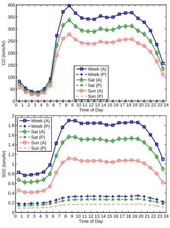
The emission inventory used for CO and SO₂ is based onWest et al. (2004) with updated totals fromComisi ´on Ambiental Metropolitana(2004). The spatial pattern of the CO area sources is shown in Fig.2a, and the point sources in Fig. 2c. The SO₂ emissions are shown in Figs.2b and d. The temporal profile of both CO and SO₂ is shown in Fig.3. This shows that the point sources are negligible for CO and small for

15

SO₂, although including the Tula industrial complex and Popocat ´epetl volcano would change this picture. There is a clear peak at the morning rush hour, sustained traffic throughout the day and reduced emissions at night.

Stochastic particle trajectories are calculated using FLEXPART (Stohl et al.,2005), as described inde Foy et al.(2006c). Backward trajectories are calculated for specific

20

fixed sites. For these cases, 100 particles per hour are released between 0 and 50 m above ground and are traced back for 48 h. Forward trajectories are calculated with the CO spatial and temporal distribution described above to provide simulated CO fields.

Residence Time Analysis was carried out using the particle simulations following Ashbaugh et al. (1985). For a one hour release, all particle positions at every hour

25

of the simulation are stored. A surface grid is applied over the simulation domain, and all particle positions in each grid cell are totalled for the entire simulation. This gives “Residence Times”, the grid corresponds to a time exposure photograph of the

(13)

ACPD

6, 6125–6181, 2006

Tables Figures

J I

Back Close

Full Screen / Esc

EGU particle tracks, with values equivalent to the length of time spent in each cell by particles

emitted.

The Residence Times can be summed for hourly releases during the whole campaign to identify preferred transport directions. In order to identify possible source regions, Concentration Fields were calculated. To derive these, Residence Times from

5

backward trajectories are summed after scaling by the surface concentration at the release site for the corresponding hour, following Seibert et al. (1994). All the grids of particle paths passing over source regions will therefore be scaled up while clean air trajectories will be scaled to zero so that the final sum will reveal potential source regions. It should be noted however that this method is not able to distinguish between

10

different points along the release path. As a result, the sensitivity of the method is much greater in terms of direction than in terms of distance from the source. Redistribution of Concentration Fields (Stohl,1996) was tested for this test case but was not able to converge on a solution and was therefore not used. This was probably because the sources are too spread out and the receptor sites to close to the urban area.

15

Eulerian pollutant transport was calculated using the Comprehensive Air-quality Model with eXtensions (CAMx,ENVIRON (2005)), version 4.20. This was run on the finest MM5 domain at 3 km resolution with the first 15 of the 23 vertical levels used in MM5. This corresponds to approximately 5200 m above ground and 440 hPa over Mexico City. Chemistry was turned offand the simulation was carried out for just CO

20

and SO₂acting as passive tracers.

Vertical diffusion is treated with parameterisations based on surface and boundary layer parameters. These were obtained from MM5 which was run with the MRF boundary layer scheme (Hong and Pan, 1996). The coefficients of O’Brien (1970) (OB70) and of the CMAQ model (Byun, 1999) were tested in CAMx, but not those based on

25

turbulent kinetic energy as this is not calculated by the MRF scheme.

CAMx version 4.20 had a number of improvements. Of particular relevance was the reduction in the horizontal diffusion and the time interpolation of the vertical diffusion coefficient. The first change led to reduced mixing, but the second led to increased

(14)

ACPD

6, 6125–6181, 2006

Tables Figures

J I

Back Close

Full Screen / Esc

EGU mixing in the morning hours. While these compensated each other to some degree,

the earlier mixing improved the concentration profiles during rush-hour.

3 Measurements

3.1 FTIR

Mobile column measurements of CO were made using Fourier Transform Infrared

5

Spectroscopy (FTIR). A medium resolution spectrometer (0.5 cm⁻¹) was used with a new 360-degree solar tracker. This system was used to evaluate a number of species both in fixed site mode and in mobile mode to evaluate point source emissions with the Solar Occultation Flux method (SOF). This study makes use of the 126 total CO columns measured between 11 April and 1 May.

10

The long-path FTIR (LP-FTIR) system at CENICA consisted of a medium resolution (1 cm⁻¹) spectrometer (Bomem MB104) coupled to a custom fabricated transmitting and receiving telescope. At the other side of the light path, a cubecorner array was mounted at a tower, making up a total folded path of 860 m (parallel to DOAS-1 described below). The system provided data with 5-min integration time continuously

15

from 22:20 on 9 March to 00:00 on 29 April, except for a 12 h gap on 11 April. Spec- tra were analyzed using the latest HITRAN database cross sections (Rothman et al., 2003) and a nonlinear fitting algorithm.

Separate long-path FTIR measurements were made at La Merced as described in Grutter et al.(2005) andGrutter(2003). A Nicolet interferometer was used with a ZnSe

20

beamsplitter operating at 0.5 cm⁻¹resolution. The liquid-nitrogen-cooled MCT detector had a working range of 600 to 4000 cm⁻¹. The equipment was mounted on top of two 4-storey buildings leading to a single path length of 426 m that was 20 m above ground level. Continuous data was available from 1 April to 4 May inclusive for 75% of the time.

As for the CENICA FTIR, the spectra were analyzed with the HITRAN cross sections

25

ofRothman et al.(2003).

(15)

ACPD

6, 6125–6181, 2006

Tables Figures

J I

Back Close

Full Screen / Esc

EGU 3.2 Zenith sky UV/Visible spectroscopy

A Mini-DOAS (Differential Optical Absorption Spectrometer) system was deployed.

This uses an Ocean Optics spectrometer with operating range of 280 to 390 nm and 0.6 nm resolution using the DOASIS (Kraus, 2001) and WinDoas (Fayt and van Roozendael,2001) retrieval software. In mobile mode, columns of SO₂ are obtained

5

along plume traverses. Multiplying the column integrated over the traverse by the average wind speed yields the emission estimates. Wind speed was measured at the ground as well as by dual beam mini-DOAS, with estimated speeds ranging from 3.4 m/s to 7.7 m/s for different traverses.

Six traverses were carried out for the Tula industrial complex on 1 May. This yielded

10

an average estimated emission rate of 4.6 kg/s of SO₂.

On the afternoons of 27 and 28 April, two traverses of the plume of the Popocat ´epetl volcano yielded an estimate of 9.5 kg/s. Daily summaries of volcanic activity are available from CENAPRED (http://www.cenapred.unam.mx/). These report between 2 and 25 low intensity exhalations of steam and gas everyday of the campaign. There were

15

occurrences of small to moderate explosions on 17 April, on 24 to 25 April and on 27 to 28 April. The last episode involved the ejection of incandescent debris to a distance of about 800 m at night and some moderate amplitude tremors. As described above, the volcano is a passively degassing eruptive volcano with continuous SO₂ emissions in the absence of any visible eruptions.

20

3.3 DOAS

The DOAS technique has been described in Platt(1994). Two long-path DOAS (LP- DOAS) systems were mounted at CENICA. SO₂ was measured by detection of the unique specific narrow-band (5 nm) absorption structures in the ultraviolet spectral range (near 300 nm). Both LP-DOAS were installed on the rooftop of the CENICA

25

building, from where light of a broadband UV/vis lightsource (Xe-short arc lamp) was projected into different directions into the open atmosphere: DOAS-1 pointed towards

(16)

ACPD

6, 6125–6181, 2006

Tables Figures

J I

Back Close

Full Screen / Esc

EGU an array of retro reflectors located in south-easterly direction (TELCEL tower), DOAS-2

pointed towards an array of retro reflectors located in south-westerly direction on top of the local hill Cerro de la Estrella. The lightbeam was folded back into each instru- ment and spectra were recorded using a Czerny-Turner type spectrometer coupled to a 1024-element PDA detector. The average height of the light path was 16 m and

5

70 m above ground, the total path length was 860 m and 4.42 km, the mean SO₂ detection limits were 0.26 ppbv and 0.15 ppbv, respectively. SO₂reference spectra were recorded by introducing a quartz cell filled with SO₂ into a DOAS lightbeam. Spectra were analysed using nonlinear least squares fitting routines byFayt and van Roozen- dael (2001) andStutz and Platt(1996). and reported concentrations are based on the

10

absorption cross section ofVandaele et al.(1994). Data was available for DOAS-1 from 06:00 on 3 April until 11:00 on 2 May and for DOAS-2 from 00:00 on 3 April to 17:45 on 11 April and from 08:40 on 18 April to 13:30 on 3 May. Other data from DOAS-1 and DOAS-2 is described inVolkamer et al.(2005b) andVolkamer et al.(2005a). At MER, a commercial DOAS system (Opsis) was installed with the same open-path as

15

the FTIR (Grutter et al.,2005) providing data at 5-min resolution from 1 April to 4 May.

3.4 Monitoring stations

The MCMA-2003 field campaign was based at the National Center for Environmen- tal Research and Training (Centro Nacional de Investigaci ´on y Capacitaci ´on Ambi- ental, CENICA) super-site. Figure 1 shows the location of the measurement sites

20

used in this study. A monitoring site measuring meteorological parameters and criteria pollutants is under continuous operation there. In addition, the CENICA mobile van with similar equipment was deployed within the grounds of a primary school in Santa Ana Tlacotenco (SATL). This is a small village on the south-eastern edge of the basin overlooking the MCMA. Surface criteria pollutant concentrations are mea-

25

sured throughout the city by the Ambient Air Monitoring Network (Red Autom ´atica de Monitoreo Atmosf ´erico, RAMA). This data was available both at the raw 1-min resolution and in 1-h averages, detailed information on all the stations is available online

(17)

ACPD

6, 6125–6181, 2006

Tables Figures

J I

Back Close

Full Screen / Esc

EGU (http://www.sma.df.gob.mx/simat/, see “Mapoteca”).

CO measurements were made using the Teledyne API model 300 CO analyser which uses the gas filter correlation method. Infrared radiation at 4.7 µm passes through a rotating gas filter wheel at 30 Hz. This cycles between the measurement cell containing nitrogen which does not affect the beam before passing through the detection cell, and

5

the reference cell containing a mixture of nitrogen and CO which saturates the beam.

SO₂measurements were made using pulsed UV fluorescence (Teledyne API models 100 and 100A). UV radiation of 214 nm is passed through the detection cell and the photomultiplier tube is fitted with a filter in the range of 220 to 240 nm.

The timezone in the MCMA was Central Standard Time (CST=UTC–6) before 6 April

10

and daylight saving time (CDT=UTC–5) thereafter. The field campaign policy specified the use of local time for data storage and analysis, a convention that will be followed here with times in CDT unless marked otherwise.

4 Carbon monoxide

Carbon monoxide is emitted mainly by mobile sources and acts as a passive tracer

15

on the time scales of the MCMA. It is therefore a useful quantity to verify the simulated transport by both Lagrangian and Eulerian models. For Lagrangian simulations, Concentration Field analysis can be used to identify possible source regions which can then be compared with known inventories. For Eulerian models, comparisons with surface measurements are used to verify model performance. Column measurements are

20

used to verify the total emissions and to identify potential adjustment factors.

4.1 Concentration field analysis

Concentration field analysis was applied to CO concentrations at three locations:

CENICA near the centre of the city, VIF to the north of the MCMA and SATL to the south. In order to increase the sensitivity of the method in the radial distance from the

25

(18)

ACPD

6, 6125–6181, 2006

Tables Figures

J I

Back Close

Full Screen / Esc

EGU source, it can be applied to multiple stations at once. In order to evaluate the limita-

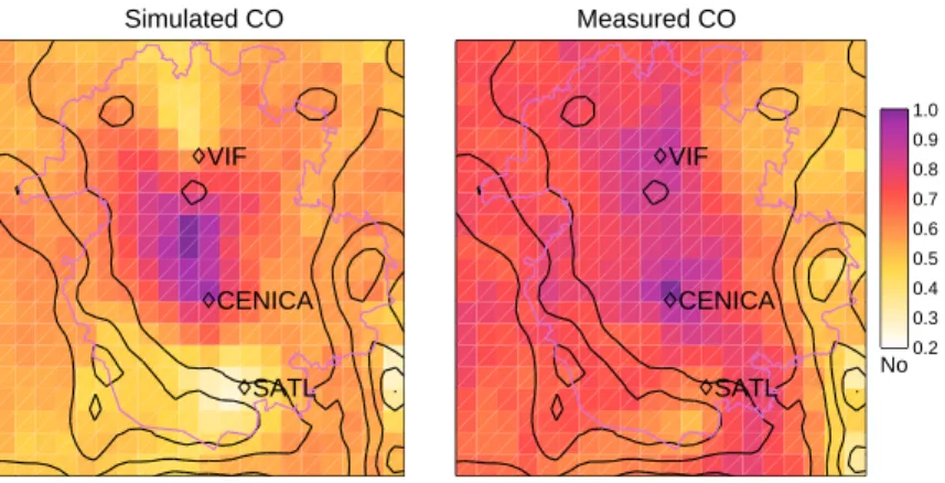
tions of the method, it is first applied to simulated concentrations obtained from forward runs of the model. Ideally, we would recover the initial emission inventory. Results are shown in Fig.4. Comparison with the spatial emission map in Fig. 2 shows that the method is able to recover the urban core of the emissions. As expected, there is

5

a high background as the method cannot distinguish distances from the observation sites. Note that this problem is reduced around VIF and SATL, and would be further reduced by adding stations all around the MCMA.

The same map with the actual measured concentrations is also shown in Fig.4. The method is still able to identify the urban emission in the centre, but the picture is much

10

less focused. There are small but noticeable impacts from wind flows from the Mexican Plateau, from the pass to Toluca and from the Chalco passage. At this point, it is not possible to say if this is due to limitations in the wind simulations, or if it is evidence of impacts from neighbouring airsheds.

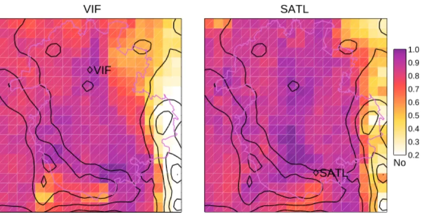
Individual Concentration Fields are shown for VIF and SATL in Fig. 5. These sta-

15

tions are removed from local emission sources and are located on the periphery of the MCMA. Results from both stations point to the MCMA urban area as the main emission source, showing that they are able to identify the direction of possible sources. Emis- sion source areas are however much more spread out for the measured concentrations than for the simulated test case, showing the limitations of the method when applied to

20

large diffuse sources that are located close to the measurement sites.

The same analysis was applied to the other RAMA stations with CO monitors. For some stations, e.g. EAC and ATI, the Concentration Fields are similar to those from VIF and SATL, pointing to the urban area. There were two different pitfalls awaiting other stations. At PED, the highest concentrations are due to local emissions during

25

times of low vertical mixing. These occurred at rush hour in the morning hours when the winds are always down hill, coming from areas with no emissions. Limiting the analysis to daylight hours when stronger winds and stronger mixing leads to more transport gave much better results. This problem can be diagnosed by first preforming

(19)

ACPD

6, 6125–6181, 2006

Tables Figures

J I

Back Close

Full Screen / Esc

EGU the analysis with model concentrations, as shown in Fig.4, which reveals the method’s

blind spots. The second pitfall is due to the presence of large local sources. These can dominate the signal at all times of the day and reduce any information content of the Concentration Fields.

4.2 Eulerian modelling

5

CAMx simulations from three test cases will be presented. Case 1 was with the OB70 vertical diffusion coefficient and case 2 with the CMAQ coefficients. Case 3 was similar to case 2 with emissions of CO scaled by a factor of 2. The minimum vertical diffusion coefficient was set to 1 m²/s for CMAQ. For OB70, the domain wide minimum was set to 0.1 m²/s and the kvpatch processor was used to reset the minimum in the bottom

10

500 m layer to 1 m²/s over urban areas and 0.5 m²/s over forests. Simulations were initialised on 31 March 2003 and run for 35 days. Emissions were scaled depending on the type of day. Saturday and Sundays had emissions that were 15% and 30% lower than weekdays. In addition, school vacation days (13 to 25 April 2003 inclusive) were reduced by 10%, Good Friday (18 April) was reduced by 50% and Maundy Thursday

15

(17 April) was reduced by 30%. Initial fields of CO were set to 0.25 ppm at the surface decreasing to 0.125 ppm at the domain top. All boundary and initial conditions for SO₂ were set to 4 ppb. These values were obtained from inspection of boundary site data as well as simulation results from the GEOS-CHEM model (Bey et al.,2001). For CO, they were verified by comparing the model predicted columns with measurements to

20

the north of the MCMA near Teotihuacan and Pachuca and outside the basin on the slopes of the Popocat ´epetl. The agreement was very good, with values ranging from 2.0×10¹⁸ to 2.5×10¹⁸molecules/cm².

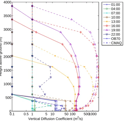
Profiles of vertical diffusion coefficients are shown in Fig. 6 for both the OB70 and CMAQ algorithms. At night, the values correspond to the specified minimum value ex-

25

cept for a shallow layer below 500 m with some mixing. The surface CMAQ coefficients are larger, but the surface layer is shallower than for OB70 and the values rapidly drop to the specified minimum value. During the day, the mixed layer develops rapidly with

(20)

ACPD

6, 6125–6181, 2006

Tables Figures

J I

Back Close

Full Screen / Esc

EGU maximum mixing reached between 16:00 and 19:00. The CMAQ coefficients are sub-

stantially higher and, more importantly, extend farther upwards than OB70. By 22:00, mixing has returned to the night-time norm although CMAQ has residual mixing in a layer aloft.

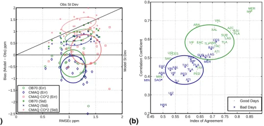
The statistical performance of the three cases is shown in Fig.7a using the statisti-

5

cal diagram introduced inde Foy et al.(2006b). The bias is plotted versus the centred root mean square error (RMSEc, also called Standard Deviation of Errors) for each RAMA CO monitor for the 34 day period from 1 April to 4 May 2003. Also plotted is the standard variation of the model versus that of the measurements, so as to evaluate the variability of the model concentrations and also to provide a comparison point

10

for the RMSEc values. These show that the OB70 case has the best fit. The CMAQ case has concentrations that are too low. Increasing the emissions removes the bias but leads to higher errors. Figure7b shows the correlation coefficient and the index of agreement (Willmott, 1982) split by episode. Model performance varied substan- tially across the different days of the campaign. The campaign was therefore split into

15

15 days that performed well (“Good CO”) and 19 days that did less well. “Good CO”

days were: 13 to 16 April and 23 April to 4 May excluding 27 April. This includes both O3-South events and the second, and longest, O3-North event. The poorly perform- ing days include the three Cold Surge episodes as well as the first O3-North episode which was the one that followed a period of heavy rains. This suggests that the current

20

model configuration performed better under dry conditions with clear skies and vigor- ous vertical mixing. Days with cloud and precipitation as well as low Bowen ratios were the poor performers suggesting that further developments will be needed to simulate evapo-transpiration and vertical mixing under more stable conditions. On this graph, the stations are labelled and show a large range of behaviour. MER and IMP are the

25

most accurately represented by a wide margin. These are city centre locations with large emissions surrounding them. Nonetheless, MER is located in a school and IMP in a campus-like environment which shield them from strong sources in the immediate vicinity. Poor performers include stations in the south such as PED and TAX. For PED,

(21)

ACPD

6, 6125–6181, 2006

Tables Figures

J I

Back Close

Full Screen / Esc

EGU the poor performance may be due to shifting emission patterns whereas for TAX it may

be due to local sources as this station is located in a major bus transport hub. The statistics diagram can also suggest possible problem areas. Both MIN and SAG are near stations that perform well (MER and XAL, respectively) although their statistics are noticeably worse. This may be due to very local effects that impact one station

5

but not its neighbour – whether due to emissions near-by or to micro-meteorological impacts.

4.2.1 Column measurements

While the statistics suggest that the current emissions with the OB70 scheme perform well, a vertical measurement is necessary to constrain the total emissions.

10

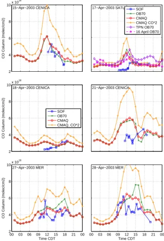
This is provided by the solar FTIR measurements which give a total column count of CO molecules per square centimetre. Figure 8 shows comparisons of measured CO columns with model predicted columns for the three cases. An offset of 0.52×10¹⁸molecules/cm² was applied to the model columns to account for the CO above the domain top, based on a free troposphere concentration of 125 ppb.

15

Agreement between model and observations is particularly good on 15 April. Unlike many urban areas where the columns increase throughout the day, CENICA experi- ences a steady reduction starting at noon. This is well captured by the model and is due to the increased horizontal wind speed diluting the urban airmass. The cases with the standard emissions both have a good fit with the column observations even though

20

their surface concentration predictions are quite different. The case with increased emissions clearly leads to too much CO in the atmosphere. There was a sharp drop in emissions on 18 April which was Good Friday, a day when all schools and businesses are closed. This can be seen in the measurements and is correctly captured by a 50%

scaling factor in the model. The model does not get the slow but steady increase dur-

25

ing the day. This is probably because the temporal distribution used was not modified and the emissions followed the usual rush hour pattern. Subjective experience on the day suggests that the city was very quiet in the morning but activity increased steadily

(22)

ACPD

6, 6125–6181, 2006

Tables Figures

J I

Back Close

Full Screen / Esc

EGU during the day. Agreement on 21 April is not nearly as good. This is attributable to the

fact that this is a Cold Surge day, with heavy clouds and some rainfall. Performance of the meteorological model was noticeably reduced during such events.

At Santa Ana, the observations show a sharp increase after noon when the urban plume reaches the southern basin rim. In contrast, the model felt the plume several

5

hours earlier and then returned to background levels with the development of the wind jet through the Chalco passage. Columns 20 km to the west at TPN show a later peak and higher values in the afternoon. Likewise, SATL columns the day before (16 April) also show a later peak. This suggests that the discrepancy is caused by too strong southward transport in the morning and too strong a jet from the Chalco passage in

10

the model, but that nonetheless the flow features can be represented by the model.

Finally, columns at La Merced show that the simulated columns of CO are indeed at the right level without any adjustments in emissions. The columns rise and fall under the competing impact of traffic and wind transport. The greater variability of the measurements is probably due to sub-grid scale effects from a combination of local CO

15

sources and small-scale wind fluctuations.

4.2.2 Spatial analysis

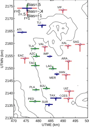
Based on the analysis above, the case with unchanged emissions and OB70 vertical diffusion will be retained as the base case for further analysis. Figure9shows the bias and error for each station for the 15 days of the “Good CO” episodes. A clear pattern

20

emerges, with positive bias (simulations higher than measurements) for central and south-western stations and negative bias for northern and eastern stations. This can be explained in terms of the growth of the city. The city is constrained on the southern and western edge by the slopes of the basin rim. This leaves growth on the basin floor to the east and especially to the north. The correlation coefficient is highest (smaller

25

bars) in the city centre and decreases on the periphery. While this could be due in part to the stronger signal in the city centre, it may also be indicative of changing spatial emission patterns. In this case, the temporal distribution pattern is also important.

(23)

ACPD

6, 6125–6181, 2006

Tables Figures

J I

Back Close

Full Screen / Esc

EGU Regions far from the urban centre have different driving profiles from the centre but

also from each other due to socio-economic variations.

Boxplots of simulated and measured CO concentrations for CENICA and MER are shown in Fig.10. At MER there is good agreement between the RAMA measurements, the FTIR and the model simulations. CO levels measured by FTIR in the afternoon are

5

lower than the surface RAMA measurements which may be due to the long path of the FTIR. The model simulations lie in between although they should be closer to the long path measurements as they represent a 3 km wide grid cell. At CENICA, the early morning peak is clearly captured by all the measurements. As expected, the open path measurements are lower than the RAMA point measurements. During the rest of the

10

day, the FTIR measurements are higher than the CENICA data but comparable to the RAMA data. This discrepancy should be investigated, especially if the measurements are used for validating the emissions inventory. The CAMx simulation underpredicts the concentrations especially in the morning. This is due to the fact that CENICA is on the edge of the area of high mobile emissions in the current emission inventory. A

15

revised spatial distribution is needed to improve the agreement.

Further diurnal profiles for XAL, AZC, PED and VIF are shown in Fig.11. At XAL, the pattern is well-captured but the predictions are too low. This is particularly acute in the morning with a delay in the rise of predicted concentrations. At PED, the opposite is true, with too high emissions in the early morning. VIF, to the north of the city, has much

20

lower concentrations. Nonetheless, they are under-predicted by the model suggesting that the emission inventory needs to be expanded to the north.

At AZC, the morning peak starts too soon and rises too high. This illustrates the pitfalls of comparing gridded model results with point measurements. At VAL (not shown), the timing is correct but it drops offmuch faster than the measurements. As it stands,

25

the model simulation at AZC is in better agreement with the measurements at VAL and the simulation at VAL with the measurements at AZC. Improved metrics could be obtained either by doing a cross-comparison or by comparing the average of the model with the average of the measurements.

(24)

ACPD

6, 6125–6181, 2006

Tables Figures

J I

Back Close

Full Screen / Esc

EGU 4.3 Discussion

Because of differences in vertical pollutant concentrations, surface measurements alone are an insufficient means of verifying emission levels of CO. Column measurements provide a necessary constraint on the vertical distribution of pollutants which can be used together with the surface measurements to select appropriate vertical dif-

5

fusion scheme and hence verify the emission inventory. Because CO can be treated as an inert tracer, it is possible to validate the wind transport from numerical simulations.

This can then be applied to all the species in the model.

By using both forward Eulerian modelling and backward Lagrangian trajectories and combining these with surface observations it is possible to evaluate the spatial distribu-

10

tion of the inventory. This method can suggest possible improvements on the scale of sectors of the city comprising dozens of grid cells. It is still relatively crude however and will not be able to resolve features on the scale of individual grid cells. Comparisons of diurnal boxplots at individual stations can be used to evaluate the temporal distribution of the emissions and to suggest modifications by time of day. These temporal profiles

15

vary spatially and can be observed at different stations throughout the city.

Varying emissions during vacations and holidays are an additional source of uncertainty and model under-performance that has not been quantified in the present study.

Scaling factors for high and low emission days can be deduced from CO observations.

Caution must be exercised as peak CO is representative of emissions preceding the

20

growth of the mixing layer and does not distinguish between emission levels later in the day. The biggest change by day of week and type of day may be the temporal distribution rather than the overall emission level. Further work will need to refine this with traffic count data that can resolve the spatial differences within the MCMA.

(25)

ACPD

6, 6125–6181, 2006

Tables Figures

J I

Back Close

Full Screen / Esc

EGU 5 Sulfur dioxide

5.1 Concentration field analysis

Concentration field analysis was performed for SO₂ in the same way as for CO, see Sect.4. Results for VIF and SATL, the stations most to the north and south respectively, are shown in Fig.12. Both of these point to a focused source to the northwest of the

5

city. The signal at VIF is particularly clear, with only a small contributions from areas southwest of the station. Because SATL is further away and on the southern edge of the basin rim, the picture is more diffuse. The trace from the northwest is still clearly visible however, with suggested transport southwards along the western edge of the basin.

10

5.2 Eulerian modelling

CAMx simulations of SO₂ were carried out with the OB70 vertical diffusion scheme.

In addition to the point and area sources from the emissions inventory, point sources for the Tula industrial complex and for the Popocat ´epetl volcano were added as described in Sect.3. Generic stack parameters were used which do not affect the long

15

range transport of the plume. Emissions were set to 5 kg/s for Tula and 10 kg/s for Popocat ´epetl and were constant in time.

Figure13shows time series at VIF to the north of the city and CENICA to the south- east. In addition to the total measured and simulated SO₂, the simulated contribution of the Tula industrial complex and the volcano are shown. These were calculated sepa-

20

rately by simulating individual tracers for each source. Sharp peaks caused by plumes from the large point sources can be clearly seen. At VIF, there are 7 of these above 50 ppb during the campaign. By the time they reach CENICA, their impact is reduced except for events occurring during Cold Surge episodes when vertical mixing is low and transport is directly from the north. The volcano has the potential to impact the city

25

even during the dry season when winds aloft are predominantly westerly. The signal is