HAL Id: hal-00288222
https://hal.archives-ouvertes.fr/hal-00288222
Submitted on 16 Jun 2008
HAL is a multi-disciplinary open access archive for the deposit and dissemination of sci- entific research documents, whether they are pub- lished or not. The documents may come from teaching and research institutions in France or abroad, or from public or private research centers.
L’archive ouverte pluridisciplinaire HAL, est destinée au dépôt et à la diffusion de documents scientifiques de niveau recherche, publiés ou non, émanant des établissements d’enseignement et de recherche français ou étrangers, des laboratoires publics ou privés.
The modular decomposition of countable graphs : Definition and construction in monadic second-order
logic
Bruno Courcelle, Christian Delhommé
To cite this version:
Bruno Courcelle, Christian Delhommé. The modular decomposition of countable graphs : Definition and construction in monadic second-order logic. Theoretical Computer Science, Elsevier, 2008, 394, pp.1-38. �hal-00288222�
DEFINITION AND CONSTRUCTION IN MONADIC SECOND-ORDER LOGIC
BRUNO COURCELLE AND CHRISTIAN DELHOMM ´E
Abstract. We consider the notion of modular decomposition for countable graphs. The modular decomposition of a graph given with an enumeration of its set of vertices, can be defined by formulas of Monadic Second-Order logic.
Another result is the definition of a representation of modular decompositions by low degree relational structures. Such relational structures can also be defined in the considered graph by monadic second-order formulas.
1. Introduction
Finite and infinite trees and graphs can be studied from different points of view : as binary relations, as generalized words to which the methods of formal language theory can be applied or asalgorithmic objects. These perspectives are developped respectively in the book ontheory of relations by Fra¨ıss´e [29], in the book chapter by Courcelle [14] for the extension of language theory to finite graphs, in many books on graph algorithms, among which we quote the one by Downey and Fellows onparametrized complexity[25]. The study of infinite trees and graphs is motivated by the need offormalizing the semantics of programs and of processes in order to verify them [9, 12, 20], and by research on combinatorial group theory [39, 43].
However it is an interesting chapter of graph theory on its own, see for instance the book by Diestel [24].
Algorithms and decidability questions are meaningful for finite graphs and for infinite graphs described in finitary ways. Many types of finite descriptions of countable graphs have been proposed : by pushdown automata and more generally by languages [42, 5], by equation systems [10, 1], by automatic structures [33, 38, 3], by formulas of monadic second-order logic [10, 4]. The doctoral dissertation of T. Colcombet [6] presents a detailed comparison of these different specification methods.
Two importants tools for all these studies aregraph decompositionsandmonadic second-order logic. Graphs, finite as well as infinite, can be decomposed in several ways. By adecompositionof a graph, we mean a construction of this graph that uses a specified set of basic graphs and graph composition operations. For instance a graph is obtained from its biconnected components by one-vertex gluings. Another
Date: November 8, 2007.
Key words and phrases. Modular decomposition, Tree, Linear order, Monadic second-order logic, Monadic second order transduction.
Acknowledgement : This work has been initiated during a stay of B. Courcelle in the ERMIT group, in 2004, supported by the University of La R´eunion. It has also been supported by the project GRAAL of the ”Agence Nationale pour la Recherche”.
1
example is the very well-known notion oftree-decomposition. The global structure of a decomposition is always a tree.
Graph decompositions are very useful for the understanding of the structure of certain types of graphs and also for algorithmic purposes. In particular, the notions of tree-decomposition and oftree-widthare fundamental for the construction offixed parameter tractable algorithms for many problems, in particular for NP-complete ones. Many such problems have polynomial time algorithms on graphs of tree-width at mostk. This use of tree-decompositions is developped in the book [25]. Clique- width is another graph complexity measure on graphs, based on the expression of a graph from one-vertex graphs by means of certain graph operations, and that is interesting for algorithmic purposes ([21]). For graphs of bounded tree-width or of bounded clique-width, efficient algorithms can be obtained for problems expressed inmonadic second-order logic.
The present article investigates the modular decomposition of infinite (mainly countable) graphs. The notion of modular decomposition of a finite graph has been studied extensively in many articles, and under various names. M¨orhing and Radermacher give in [41] a survey of this frequently rediscovered notion. The composition operation underlying its definition is the substitution of a graph H for a vertex v in a graph G. In the resulting graph, denoted by G[H/v], the vertex v is replaced by H, and all its neighbours in G are linked to all vertices of H. A subgraph H of a graph K is a module if K is of the form G[H/v].
Among those are distinguished thestrongmodules, namely those modules that are comparable for inclusion with every module that they meet. The strong modules form a finite tree where the ancestor relation is inclusion (X ⊆Y if and only ifY is an ancestor ofX). This tree is called itsmodular decomposition. It corresponds to a canonical expression of the graph in terms of (nested) substitutions. Furthermore, this decomposition can be constructed from the given graph by monadic second- order formulas, as proved in [13]. This result enriches the logical tool box and helps to express graph properties in monadic second-order logic, which yields, ultimately, polynomial algorithms and decidability results (see [42, 10, 14] for decidability results based on monadic second-order logic).
The notion of modular decomposition is essential, not only for algorithmic pur- poses, but also for establishing structural properties of graphs and related objects, in particular of partial orders and their comparability graphs. For instance, one can compute the number of transitive orientations of a finite comparability graph from its modular decomposition. Motivated by the investigation of comparability graphs, and in particular for proving that the dimension of a partial order depends only on its comparability graph, Kelly [37] reviews Gallai’s fundamental analysis of the properties of modules of finite undirected graphs [30] and extends it to infinite ones. The strong modules of an infinite graph are pairwise disjoint or comparable for inclusion, but they do not form a tree in the usual sense where a tree is de- fined as a connected and directed graph without circuits such that every vertex is reachable by a unique directed path from theroot (the unique vertex of indegree 0). They form a tree provided one defines atree as a partial order such that the set of elements larger than any element is linearly ordered, which we will do in this article. Such trees may have no root. The ordered setQof rational numbers, like any linear order, is a tree in this sense. It has no root, and no element has a father because no rational number has a successor.
Our aims are to define and to study modular decompositions of countable graphs, to represent them by relational structures, and to useMonadic Second-Order logic (MS logic in short)to construct from a graph certain representations of its modular decomposition by relational structures. MS logic has already been used for such constructions by Courcelle in [13], in the case of finite graphs, and our constructions build upon those of this article, with the necessity of new features for handling infinite graphs.
For defining the modular decomposition of a countable graph, we do not take all strong modules, but only some of them. Doing so we obtain a countable object associated with a countable graph. By defining the modular decomposition as the tree of all strong modules, we would obtain in certain cases an uncountable tree associated with a countable graph. This would not be satisfactory because we consider that the modular decomposition must be a synthetic representation of a graph : so it is not acceptable that it is of larger cardinality than the considered graph. There are two key tools for our study of modular decomposition of infinite graphs. On the one hand, the notion ofrobust module (already considered in [37]), defined as the intersection of all strong modules containing two vertices. And on the other hand, thecharacterization of graphs with no non-trivial strong modules1; the finite and undirected case appears in [30], and the extension to infinite directed graphs, for which we provide a somewhat simpler proof, is in Ehrenfeucht and al. [27].
Another concern is to describedense graphs,i.e. graphs having ”lots of edges”, by relational structures, actually vertex- and edge-labelled graphs, which are as sparse as possible. A finite partial order can be represented by its Hasse diagram, and this representation can be used for expressing its properties in monadic second- order logic. This is no longer the case of infinite partial orders. Consider for instance the ordered setQ. However, it can be defined as a certain ordering of the nodes of the complete infinite binary tree (here ”tree” is taken in the usual sense of computer science). This observation extends to all countable linearly ordered sets.
Furthermore, first-order formulas using an auxiliary enumeration of the considered linear orderA,i.e.an auxiliary ordering ofAisomorphic to the ordinalωcan define the representing binary tree (these formulas do not depend onA). It follows that this representation of linear orders by binary trees fits with the expression of their properties by monadic second-order formulas. We use this fact to represent the modular decomposition of a countable graphGby a countable graph of maximum degreem+3 wheremis the least upper bound of the degrees of theprime subgraphs ofG. It may happen thatmis finite, even ifGhas vertices of infinite degree. This is the case for cographs.
This article is an expanded version of [19]. It is organized in nine sections : (1) Introduction.
(2) Review of the modular decomposition for finite graphs.
(3) Basics about trees.
(4) Strong and robust modules.
(5) The modular decomposition.
(6) Construction of the modular decomposition in monadic second order logic.
1Those are the prime graphs, the undirected complete or edge-free graphs, and the linear orders.
(7) Representation of modular decompositions by low degree relational struc- tures.
(8) Concluding remarks.
(9) Appendix : Monadic second order logic and monadic second order trans- ductions.
2. Prologue : Graph substitutions and the Modular decomposition of finite graphs
This section is a quick review of the notion of modular decomposition for finite graphs and a presentation of our view of this notion, in the perspective of its extension to countable graphs.
Graphs are loop-free without multiple edges. A graphGis handled as a relational structurehVG, edgGi. Its domain is the vertex setVGandedgGis a binary relation such that edgG(x, x) never holds. We write also x −→G y if edgG(x, y) holds. A graph is undirected if for every vertices x and y, x −→G y implies y −→G x ; it is directed if x −→G y and y −→G x never hold simultaneously. It is total if any two distinct vertices are linked by an edge. It iscomplete if it is total and undirected.
We say that a graph is alinear order if for some strict linear ordering < onVG, x−→G y if and only ifx < y.
We denote by G[X] the induced subgraph of G with vertex set X ⊆ VG. A graphH embedsinto a graphGifHis isomorphic to an induced subgraph ofG.
2.1. Graph substitution and modules.
Definition 2.1. (Graph substitution.) Let K be a graph and let (Hv)v∈VK be a family of pairwise disjoint graphs (they have no vertex in common). We denote by K[Hv/v;v ∈VK] the graphG resulting from the simultaneous substitution ofHv forv∈VK. It is defined as follows
• VG=∪{VHv :v∈VK}
• u−→G u0 if and only if
– eitheru−−→Hv u0 (withu, u0∈VHv) for somev,
– or there are two distinct v, v0 ∈VK such that v 6=v0, u∈VHv, u0 ∈ VHv0 andv−→K v0.
Notation 2.1. If, in that definition, K is an edge-free graph we write G =
⊕v∈VKHv and we say thatGis thefree sumof the family (Hv)v∈VK.
If K is a complete graph we write G = ⊗v∈VKHv and we say that G is the complete sumof the family (Hv)v∈VK.
If K is a linear order (VK, <) (thus v −→K v0 if and only if v < v0), we write G=−→
⊗v∈VKHv and we say thatGis thelinear sumof the family (Hv)v∈VK where the set of indicesVK is linearly ordered by<.
As binary operations,⊕and⊗are associative and commutative, and the oper- ation−→
⊗ is only associative.
Definition 2.2. (Modular partition, module.) In order to characterize the ways in which a graphG can be expressed asK[Hv/v;v ∈VK], one defines the notion of modular partition: it is a partition C of the vertex setVG (the members ofC are pairwise disjoint non-empty sets of vertices, of which the union is the vertex set) such that for any two distinctM andN in Cand anyu, u0∈M,v, v0 ∈N
u−→G v if and only ifu0 −→G v0
Each memberM ofCis amodule,i.e.a set of vertices such that for anyu∈VG\M for anyv, v0 ∈M
(u−→G v if and only ifu−→G v0) and (v−→G uif and only ifv0−→G u)
The sets ∅, VG and {v}for each v ∈ VG are modules and are called the trivial modules.
IfC is a modular partition, then thequotientis the graphK=G/Cdefined by : (1) VK=C
(2) M−→K N if and only if for someu,v we haveu∈M,v∈N andu−→G v.
From the definitions it follows immediately :
Proposition 2.1. (1) If G = K[Hv/v;v ∈ VK], then the sets VHv form a modular partition of G.
(2) If C is a modular partition ofG, thenG= (G/C)[H[M]/M;M∈ C].
We may also consider as modular partition any indexed partitionC= (Vi)i∈I (in particular theVi’s are pairwise distinct) such that{Vi:i∈I}is a modular partition in the sense above ; thus the set of vertices ofG/CisI, andG= (G/C)[H[Vi]/i;i∈ I].
2.2. Decompositions. LetG be a graph expressed asK[Hv/v;v∈VK]. We say that this expression defines a decomposition ofGinto the graphsHv,v∈VK. The graphsHv may themselves be decomposed into smaller graphs, which themselves may be decomposed similarly. Thus we obtain a notion of graph decomposition, that can be defined as follows.
Definition 2.3. (Decompositions.) Two sets Aand B meet ifA∩B 6=∅; they overlap ifA∩B6=∅,A\B6=∅andB\A6=∅.
Adecomposition2 of a graphG is a familyDof subsets ofVG such that (1) ∅6∈ D,VG∈ D,{v} ∈ Dfor eachv∈VG ;
(2) no two members ofDoverlap ;
(3) for every M ∈ D, letting mp(M,D) denote the set of maximal proper subsets ofM that belong toD, ifmp(M,D) is non-empty then it forms a modular partition ofG[M] denoted byπ(M) (orπD(M) when Dneed to be specified).
Hence ifG=K[Hv/v;v∈VK], the family
D={VG} ∪ {VHv :v∈VK} ∪ {{v}:v∈VG}
is a decomposition of G. If furthermore Dv is a decomposition of Hv for each v∈VK, then
D0=∪{Dv:v∈VK} ∪ {VG}
is a decomposition ofGthat refinesD, that is, such thatD ⊆ D0.
Let us conversely assume that Dis a decomposition of a graphG. By the first two conditions, (D,⊆) is a tree, denoted byT ree(D) : its nodes are the elements ofD,X (Y if and only ifY is an ancestor ofX,VGis the root and the singletons {v}are the leaves.
Because of the finiteness of D, a set mp(M,D) is not empty except whenM is a leaf. It follows that for eachM∈ Dthat is not a leaf,
G[M] = (G[M]/π(M))[G[N1]/1, . . . ,G[Nn]/n]
whereN1,. . ., Nn are the sons ofM in T ree(D). In particular G= (G/π(VG))[G[N1]/1, . . . ,G[Nn]/n]
2From now on, the word ”decomposition” will be used in the sense of this definition.
whereN1,. . ., Nn are the sons of the root.
Lemma 2.1. LetDbe a decomposition of a finite graphG, letN1, . . ., Nn be the sons ofVG in the tree ofD. Then for eachi,{X∈ D:X ⊆Ni}is a decomposition of G[Ni].
It follows that every decomposition D of a finite graphG yields an expression ED of that graph in terms of nested substitutions of the graphs G[M]/π(M) for M∈ D. The graphsG[M]/π(M) are called thefactorsof the decomposition.
Conversely with every expressionE of a finite graph G in terms of nested sub- stitutions of graphs is associated a decompositionDsuch thatED=E.
A graph has several decompositions. However a canonical one, called the modular decomposition, can be defined.
Definition 2.4. Strong modules. The modular decomposition of a finite graph.
A module in a graph is strong if it is non-empty and overlaps no module. The set of strong modules of a finite graphG is a decompositionDcalled itsmodular decomposition. We will identify that set of strong modules and the corresponding tree, that we will denotemdec(G).
The quotient graphsG[M]/π(M) forM ∈ D,M not singleton have a particular structure described by the followingFundamental Theorem of Modular Decomposi- tion. A graph isprimeif it has no non-trivial module and at least three vertices.
Theorem 2.1. For every finite graph G with at least two vertices, if π is its modular partition into maximal proper strong modules, then G/π has at least two vertices and has one of the following forms :
(1) either it is edge-free (2) or it is complete (3) or it is a linear order (4) or it is prime
The graph G has one and only one of the following forms, respectively : (I) G=H1⊕ · · · ⊕Hn, n≥2, where no Hi is a free sum.
(II) G=H1⊗ · · · ⊗Hn, n≥2, where no Hi is a complete sum.
(III) G=H1−→
⊗ · · ·−→
⊗Hn,n≥2, where noHi is a linear sum.
(IV) G=P[H1/v1, . . . ,Hn/vn]wherePis a prime graph and n≥3.
It follows that each node M of the modular decomposition which is not a leaf has type I, II, III or IV, corresponding respectively to the expression of G[M] of one of the above forms with Hi =G[Ni] where N1, . . ., Nn are the sons of M in the treemdec(G). IfGis undirected, then case III does not occur and furthermore n ≥ 4 in case IV because the smallest prime undirected graph is the undirected path with 4 vertices.
That theorem seems to have been rediscovered many times. For finite undirected graphs, Kelly [37] attributes it to Gallai [30]. For the case of directed graphs, generalizations and references, we refer the reader to [28, 32, 40, 41]. M¨ohring and Radermacher [41] call ”substitution decomposition” the modular decomposition and thus emphasize its relation with graph substitution. They show that analogous decompositions can be defined for other discrete structures like hypergraphs and Boolean functions. The structure of prime graphs is investigated by Ille in [36, 35], which improve previous results by Ehrenfeucht and Rozenberg [26] and Schmerl and Trotter [44].
The graphs for which all nodes of the modular decomposition are of the forms (I) or (II) are called cographs ; those are precisely the simple undirected graphs without induced path with 4 vertices.
2.3. Representing decompositions by binary structures. Relational struc- tures and logic are reviewed in the appendix. A binary structure is a relational structure all relations of which are unary or binary. As said above, a graphG is considered as the binary structurehVG, edgGi. It is undirected if and only ifedgGis symmetric. We consider only graphs without loops, henceedgG(x, x) never holds.
We have defined a decomposition Dof a graphG as a family of subsets of the vertex set VG. Such an object is not a relational structure. However, a decom- position is a tree (for inclusion as ancestor relation). Hence we can represent it by a relational structurehNT,≤Tiwhere NT is in bijection by, sayh, with Dand x ≤T y iffh(x)⊆h(y). Hence T is the tree T ree(D). The vertex set VG is then in bijection with the set of leaves of T, because {v} ∈ D for every v ∈VG. This bijection is defined byh(x) ={v}forx∈NT andv∈VG.
The graphGcannot be determined from this binary structure. We will expand it into a richer binary structure by adding unary and binary relations representing the structure of nodes,i.e.the graphsG[M]/πD(M) for the nodesM ofT ree(D).
We obtain in this way a binary structure that can be considered as a labeled graph.
Definition 2.5. The graph representation of the modular decomposition. Let G be a finite graph andDits modular decomposition. Thegraph representationofD is the binary structure
Gdec(G) =hNT,≤T, lab⊕, lab⊗, lab−→⊗, f edgi wherehNT,≤Tiis as above,T =T ree(D),
• lab⊕(x) holds if and only ifxis a node of type (I),i.e., defines a free sum,
• lab⊗(x) holds if and only ifx is a node of type (II),i.e., defines a complete sum,
• lab−→⊗(x) holds if and only if x is a node of type (III),i.e., defines a linear sum,
• f edg(x, y) holds if and only ifxandy are two sons of a nodezof type (III) or (IV) such thatx →y in the graphG[M(z)]/πD(z), whereM(z) is the corresponding module.
The prefixf inf edgrecalls that we deal with the edges of certain factors of the modular decomposition and not with the edges of the graphG.
Ifzhas label−→
⊗, i.e.is of type III, thenf edglinearly orders its set of sons. Ifz has no label and is not a leaf, then it is of type IV andf edg represents the edges of the corresponding prime factorG[M(z)]/πD(z).
The structureGdec(G) is somewhat redundant. One could delete the labelling of nodes of type III, because the distinction between types III and IV can be made from the relation f edg. However, we think more clear to have a specific labelling for these nodes.
For a cograph, the structure Gdec(G) reduces to hNT,≤T, lab⊕, lab⊗i which represents a term over the operation symbols⊕and⊗and the constant1. Since⊕ and⊗are associative and commutative, they are handled as functions of variable arity (at least 2) and unordered set of arguments.
Proposition 2.2. Every graph can be defined from the graph representation of its modular decomposition.
Proof. LetG be a finite graph and
Gdec(G) =hNT,≤T, lab⊕, lab⊗, lab−→⊗, f edgi.
ThenG=hVG, edgGican be defined as follows :
VG={x∈NT :y <T xfor noy∈NT}
edgG(x, y) holds if and only ifx, y∈VG,x6=yand, lettingzbe their least common ancestor in the treeT,
• eitherlab⊗(z) holds
• or¬(lab⊕(z)∨lab⊗(z)) holds andf edg(x0, y0), where x0, y0 are the (neces- sarily) distinct sons ofzsuch thatx≤T x0,y≤T y0
The correctness of this definition follows immediately form the definitions From that proof it is clear thatG can be reconstructed fromGdec(G) by first- order formulas. It is proved by Courcelle [13] that Gdec(G) can be constructed from G by monadic second-order formulas, with the help of an auxiliary linear ordering4ofVG.
Our objectives will be the following ones :
• to extend the definition of modular decomposition to infinite graphs ;
• to extend the above result of [13] to countable graphs given with an auxiliary linear ordering of typeω of the vertex set ;
• to replace the binary structureGdec(G) by an alternative binary structure, called its sparse representation, which, considered as a graph, has vertices of ”low degree”.
3. Trees
In the present Section, no particular assumptions of cardinality are made.
Definitions 3.1. (Trees, join-trees and leafy trees.) Our terminology borrows from R. Fra¨ıss´e [29], with some variations.
Given a partially ordered set (P,≤), two elements x andy ∈P arecomparable if x ≤y or y ≤x, they arecompatible if the pair {x, y} has an upper-bound. A chainis a set of pairwise comparable vertices. A setQ⊆P of vertices is (upwards) directedif
∀x, y∈Q, ∃z∈Q, x≤z∧y≤z A setQis anup-set(resp. down-set)if
∀x∈Q, ∀y∈P, x≤y⇒y∈Q(resp. ∀x∈Q, ∀y∈P, x≥y⇒y∈Q).
We will use the following notation : Px={y∈P :x≤y},P>x={y∈P :y > x}, Px={y∈P:y≤x}and P<x={y∈P:y < x}.
A forest is a partial order (T,≤) such that for everyx∈T, the setTxis a chain ; the elements ofT are callednodes. Atreeis a forest that isdirected. In a forest, the relation of compatibility is an equivalence whose classes are called thecomponents ofT. The components are the maximal directed sets ; they are also the connected components of the comparability graph.
A tree is ajoin-tree if any two nodes x andy have a least upper bound, called theirjoinand denoted byx∨y. A join-tree can be defined as a relational structure (T,≤) or as an algebraic structure (T,∨), withx ≤y if and only ify =x∨y. A sub-join-tree of (T,≤) is a tree (T0,≤0) with T0 ⊆ T and, for any x and y in T0, x∨0y=x∨y (so in particularx≤0y if and only ifx≤y).
Aleaf in a forest is a minimal node, aroot is a maximal one. Aninternal node is one that is not a leaf. A forest may have one or several roots, or no root at all. It may have no leaf. A tree has at most one root. We say that a tree isleafy if every internal node is the least upper bound of two leaves. Notice that every leafy tree is a join-tree. A finite tree is a finite rooted tree in the usual sense, and its root is the unique maximal element. A finite forest is a finite free sum of finite trees.
Ifx≤y, we say that the nodey is anancestor of x. We say thatyis the father ofxif it is the least node among those greater thanx; in that case, we say thatx is ason ofy.
Definition 3.2. (Directions in forests.) LetT be a forest. For every nodex,T<x
ordered by the induced ordering, is a forest, hence a free sum of trees. Each of these treesD is called adirection relative to x.3 Fory ∈D, we say thatD is the direction of y relative to x. We denote it bydirx(y). We denote byDir(x, T) the set of directions relative tox. Thus the directions relative toxare the components ofT<x.
Thedegree of a nodex is the cardinality ofDir(x, T). A tree is binary if every node has degree at most 2. If a node isy∨z where y and z are incomparable, it has degree at least 2. IfT is finite, this definition of the degree of a node yields the number of its sons.
Here are some easy facts listed for later reference : Lemma 3.1.
3We identify a direction and the corresponding set of nodes.
(1) In a tree, given two nodes in distinct directions relative to a nodex, thenx is their join ; conversely, if two incomparable nodes have a join, then they lie in distinct directions relative to it.
(2) In a tree every directed set of nodes has a cofinal chain4.
(3) In a join-tree, the least-upper bound of any three-element set is the join of a pair of these elements, indeed of at least two pairs of these elements.
(4) In a join-tree, the least-upper bound of any finite set is the join of two elements of that set.
(5) In a join-tree, of the three least upper-bounds of the pairs of a three-element set, at least two equal the greatest.
(6) In a leafy tree, if vis an upper-bound of a set X of nodes, but not the least one, then there is a leaf y such that for every x∈X, x∨y=v.
(7) In a non-empty forest, the components are the non-empty directed simul- taneously up- and down-sets, and the maximal chains are the non-empty chains that are up-sets and have no strict lower bound.5
(8) A tree is leafy if and only if every inner node has at least two directions and every non-empty down-set contains a leaf.
(9) In a tree, any two directed down-sets that meet are comparable for inclusion.
Proof.
(2) If the directed set is empty then the empty chain suits. If the directed set D is not empty, then, given anyv∈D, considerC:={u∈D:v≤u}.
(3) Given three nodes x,y and z, if x∨y < x∨y∨z, then x, y andx∨y lie in the same direction ofx∨y∨z, butx∨y∨z= (x∨y)∨z6< x∨y∨z, thusz cannot lie to the same direction (i.e. either it equalsx∨y∨z or it lies in an other direction), so that bothx∨z andy∨z equalx∨y∨z.
(4) Induction using (3) and the associativity of∨.
(5) Consequence of Point 3.
(6) Notice thatX is included in a direction ofv; any leafylying in a different direction suits.
(9) Assume thatD andD0 are two distinct directed down-sets that meet. So lety∈D∩D0and, without loss of generality,x∈D\D0, and then an upper bound zof {x, y}in the directed set D. Now given anyx0 ∈D0, consider an upper bound z0 of{x0, y}in the directed setD0 ; observe that z0 ≤z : z0 and z are comparable since both ≥ y, but z 6≤ z0 since x ≤ z and z0 belongs to the down-setD0 that excludes x ; hence x0 ≤z0 ≤z ∈D, so thatx0∈D, that is a down-set.
Lemma 3.2. Letxandybe two nodes of a tree such thaty < x, and letD denote the direction of y relative to x. The node y is a son of x if and only if it is the greatest element of D. IfD has no greatest element, then it admits a cofinal chain containing y, and x is the least upper-bound of any such chain.
4Acofinal(resp. coinitial) set of a setP of vertices of a partially ordered set is anyQ⊆P with the property that for every elementxofP, there is an elementyofQsuch thatx≤y(resp.
y≤x).
5In a partially ordered set, astrict lower-boundof a set of vertices is a vertex that is strictly smaller than every element of that set ; in other words, it is a lower bound not belonging to the set.
Proof. Observe that, ifz is a node such thaty ≤z < x, then z∈D.
Remarks 3.1. For a partially ordered set (P,≤), we letHD(P) denote itsHasse diagram,i.e.the directed graph with set of verticesP and edgesx−→y such that x < y and there is noz with x < z < y. We say that P is diagram-connected if P is the transitive closure ofHD(P) andHD(P) is connected. A tree isdiagram- connected if the graph of the father-son relation is connected ; any two nodes are then at finite distance in this graph. A diagram-connected tree may have no root.
The infinite trees representing infinite algebraic terms over finite signatures (Courcelle [8] or [9]) and the genealogies (F. Gire, M. Nivat [31]) are diagram- connected join-trees. Some infinite trees as defined in Definition 3.1 represent nei- ther infinite trees in the sense of [8], nor genealogies.
4. Strong and robust modules
4.1. The tree of strong modules. Although a forest is a graph or can be con- sidered as a graph, we use the special term ”nodes” for the vertices of a tree or a forest. This particular terminology will be useful for clarity in situations where we discuss simultaneously a graph and a tree representing it.
Modules and modular partitions are defined (Definition 2.2) in Section 2 ; recall that a module is strong if it is non-empty and it overlaps no module.
Notation 4.1. We denote bysdec(G) the set of strong modules of any graphG.
The results of Section 2 do not extend immediately to infinite graphs, because it may happen that a graph has no maximal proper strong module (see Example 4.3 below). In such a case, Theorem 2.1 does not extend. Besides, a countable graph may have uncountably many strong modules (see Example 4.4) ; still the tree of strong modules has countably many non-limit nodes. These particular nodes will be sufficient to reconstruct the tree by a kind of ”completion”.
Let us first mention the following easy facts : Lemma 4.1. In a graph,
(1) the intersection of a non-empty set of modules is a module (possibly empty) ; (2) the union of two modules that meet is a module, and more generally, the union of a set of modules is a module as soon as the meeting relation on that set is connected ;
(3) for two modulesM andN, ifM\N is non-empty, thenN\Mis a module.
Example 4.1. The modules of a chain are its intervals ; in particular the strong modules of a chain are trivial. The first assertion is clear. As for the remaining one, given a chain (C,≤), ifI is a proper interval with at least two elementsa < b, then at least one of the two intervals{x∈C:x > a}and{x∈C:x < b}overlaps I.
Example 4.2. Every connected component of a graph is a strong module.
Example 4.3. Abicoloring of a chainC= (C,≤) is a mapping χ:C→ {⊕,⊗}.
The graph associated with a bicolored chainCas above is the undirected graph on the set C such that two distinct vertices are linked if and only if the greater one is colored by⊗. (Such graphs are sometimes calledlinear cographs.) A bicoloring χ of C is good if for x < y and i ∈ {⊕,⊗}, there is z such that x ≤z ≤ y and χ(z) =i. In particular, no two consecutive vertices have the same color.
The modules of the graph associated with a good bicoloring of a chain are the singletons and the down-sets ; in particular all its modules are strong.
Any down-setI is a module, even when the bi-coloring fails to be good. Con- versely, consider the graphG associated with a good bicoloring of a chain (C,≤).
IfAis a subset ofC failing to be an interval, then it is not a module ofG : letting a < b < cwithaandc inA andb /∈A, in caseχ(b)6=χ(c),b is linked in different ways toaandc, and in caseχ(b) =χ(c), there must be a vertexdin between with a different color. If d∈M then let it play the role of c and otherwise let it play the role ofb. A non-singleton intervalA failing to be a down-set is not a module either : given a < b with b ∈A and a /∈A, consider some other element c of A, sinceA is convex,a < c; if b andc have different labels then ais linked to them in different ways, and if they have the same label, then given some d in between with a different label, thatdmust lie inA, which is assumed to be convex, and it is linked toadifferently fromc.
The chainZ of integers has exactly two good bicolorings, they are isomorphic.
The associated graphGζ is represented on Figure 1.
⊕
⊕ ⊗ ⊕ ⊗
⊗ ⊕ ⊗ ⊗
Figure 1. The graphGζ
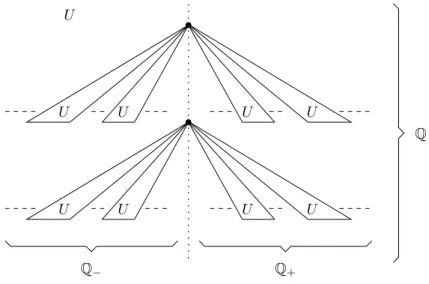
Example 4.4. The good bicolorings of the chainQof rational numbers are isomor- phic with one another ; letGη denote the associated graph. (As for the existence, one can label by⊕the rationals of the form 2mn for somem∈Zandn∈N, and by
⊗the others.)
Since Qhas uncountably many down-sets, the graph Gη is a countable graph with uncountably many strong modules.
Let us consider the basic properties of the tree of strong modules.
Lemma 4.2.
(1) The intersection of any set of strong modules is empty or is a strong module.
(2) The union of any directed set of strong modules is a strong module.
Notice that, in that statement, the intersection of the empty set is the vertex set ofG.
Proof.
(1) Let E ⊆sdec(G) with a non-empty intersection. First∩E is a module, like any intersection of a set of modules. If a set M ⊆ VG overlaps ∩E, then it overlaps some member ofE : Indeed sinceM\ ∩ E 6=∅and M\ ∩ E =
∪{M\E : E ∈ E}, there is someE ∈ E such that M\E 6= ∅, while, for any such E, E\M ⊇ (∩E)\M 6=∅. Thus ∩E overlaps no module, since no member ofE overlaps any module. Incidentally notice thatE is a chain whenever its intersection is non-empty.
(2) Let E be a directed subset ofsdec(G). If a setM⊆VG overlaps∪E, then it overlaps some member ofE : Indeed since (∪E)\M 6=∅and (∪E)\M=
∪{E\M:E∈ E}, there is someE∈ E such thatE\M6=∅, while, for any suchE,M\E⊇M\(∪E)6=∅. Thus again∪E belongs tosdec(G).
Notation 4.2. For any non-emptyA⊆VG, we letS(A) denote the intersection of all strong modules includingA; thusS(A) is the least strong module includingA.
From Lemma 4.2, it immediately follows : Corollary 4.1.
(1) sdec(G)∪ {∅}is a complete lattice. The greatest-lower bound of a subsetE of sdec(G)is its intersection ∩E ; its least upper-bound is the intersection of all members of sdec(G) including its union : W
E = ∩{S ∈sdec(G) :
∪E ⊆ S}. In particular for every non-empty subset X of VG, the least strong module includingX isS(X). The treesdec(G)of strong modules of G is a join-tree.
(2) The least upper-bound of a directed set of strong modules is its union.
(3) If D is a direction relative to some M ∈ sdec(G) then, either D has a greatest memberN in which caseN is a son ofM insdec(G), orM itself is the least upper bound ofD insdec(G).
Proof. Only (3) requires some comment : IfW
D(M, then for anyN ∈sdec(G) such that W
D ⊆ N (M, D ∪ {N}is a directed set of nodes all lesser thanM,
henceD ∪ {N} ⊆ Dby maximality of D.
The following lemma about modules of subgraphs and quotient graphs is easy to establish.
Lemma 4.3. Consider a graphG.
(1) (a) Every module of G included in a set of vertices A is a module of the induced graph G[A]. Those are the only modules of G[A] if and only ifA is a module ofG.
(b) Every strong module ofGincluded in a moduleM is a strong module ofG[M]. Those are the only ones if and only ifMis a strong module ofG.
(2) (a) LetC be a modular partition of G. The modules of the quotient graph G/Care the subsets of C whose union is a module ofG.
(b) Let C be a modular partition of G formed of strong modules. The modules of the graphG are its sets of vertices that are the union of a
module of the quotient graphG/C.
4.2. The tree of robust modules.
Notation 4.3. For possibly equal verticesxandyof a graphG, letS(x, y) denote the least strong module S({x, y}) containing x and y. We call robust any such strong module and we denote by rdec(G) the set {S(x, y) : x, y ∈ VG}. It is the tree, ordered by inclusion, of robust modules ofG.
For any distinct vertices x and y, let A(x, y) denote the union of all strong modules containingx but noty.
Notice that a module is robust if and only if it is of the form S(F) for some non-empty finite setF of vertices (see Lemma 3.1-4). It follows that that the tree rdec(G) of robust modules is a sub-join-tree of the tree of strong modules, and it is also a leafy tree.
Example 4.5. Consider the graphGη of Example 4.5. For any two distinct ra- tionals x and y, the robust module S(x, y) is the least down-set ofQ containing bothx andy, thus the down-set ofQadmitting max{x, y}as greatest element. It follows that the robust modules ofGη are the singletons and the initial intervals of Qwith a greatest element. Incidentally notice that for any two distinct rationals x < y,A(x, y) =Q<y andA(y, x) ={y}.
For any rational number x, the robust module Qx has two sons in the tree of strong modules, namely the singleton{x}andQ<x, which is not robust. The strong module corresponding to irrational cuts,i.e. those of the form{y∈Q:y < x}for some irrational numberx, are the strong modules that are neither a father nor a son in the tree of strong modules.
We use also this graph in Example 5.1.
Lemma 4.4. Consider a graph.
(1) For two distinct vertices x and y, A(x, y) is a strong module ; it is the greatest strong module containing x but noty.
(2) (a) For two distinct verticesx andy, the strong moduleA(x, y)is the son of the strong module S(x, y) containingx.
(b) For two comparable strong modulesM andN with N ( M, for any vertices x ∈ N and y ∈ M\N, N ⊆ A(x, y) ( S(x, y) ⊆ M, in particular, whenN is a son of M in the tree of strong modules, then N=A(x, y)andM =S(x, y).
(3) Every strong module is the union of a chain of robust modules.
Proof.
(1) The strong modules containingxform a chain, thusA(x, y) is the union of a chain of strong modules, and therefore it is a strong module.
(2) (a) The strong modules S(x, y) and A(x, y) both contain x, hence they are comparable. ThereforeA(x, y)(S(x, y) sincey belongs toS(x, y) but not to A(x, y). Now assume that M is a strong module such that A(x, y)⊆ M ⊆S(x, y) ; in particular x ∈ M ; if y ∈ M, then S(x, y)⊆M(and thenM=S(x, y)), and ify6∈M, thenM⊆A(x, y) (and thenM =A(x, y)). Thus A(x, y) is a son ofS(x, y).
(b) The inclusions N ⊆ A(x, y) ( S(x, y) ⊆ M hold by definition of A(x, y) andS(x, y). Thus, sinceA(x, y) and S(x, y) are strong mod- ules,N =A(x, y) and M =S(x, y) wheneverN and M are consecu- tive.
(3) Given a strong moduleM and anyx∈M, consider {S(x, y) :y∈M}.
Corollary 4.2. For a strong moduleMof a graphG, the following are equivalent : (1) M is a non-singleton robust module, i.e.M is of the form S(x, y) for two
distinctvertices.
(2) M is a father in the tree of strong modules.
(3) The degree ofM is greater than one in the tree of strong modules.
(4) The induced graph G[M]has a maximal proper strong module.
If those conditions hold :
(1’) For two elementsxandy ofM, M=S(x, y)if and only if their directions relative toM are distinct ; and the sons of M are the sets A(x, y) for all suchx andy inM.
(2’) All directions relative to M in the tree of strong modules have greatest elements, which are the sons of M ; in other words (cf.Lemma 3.2), each strong module N(M is included in a son ofM.
(4’) The maximal proper strong modules of G[M] partitionate M and are the sons ofM.
Proof. (1) implies (3), sincexandybelong to distinct directions relative toS(x, y) (Lemma 3.1-1), and the converse holds, since a strong module M of degree more than one is S(x, y) for any x and y belonging to distinct directions, which also yields the first part of (1’).
From Lemma 4.4-2 it follows that (1) and (2) are equivalent, and also that (1) implies the second part of (1’), as well as (2’).
Recall that the strong modules ofG[M] are precisely the strong modules ofG included inM (Lemma 4.1-1). It follows that (2) and (4) are equivalent, and that
(2’) and (4’) are equivalent.
Corollary 4.3. For a strong moduleM, the following are equivalent (1) M is not robust,
(2) M is a limit node in the tree of strong modules,
(3) M is the union of a chain of smaller strong (resp. robust) modules.
Proof. 1⇒3 by Lemma 4.4-3.
3⇒2 Clear.
2⇒1 Assuming that M is the least upper bound of a directed setD of strictly lesser strong modules, let us check thatM has only one direction, namely the down set generated byD(then, having degree one,Mwill not be robust by Corollary 4.2 above) : That down-set is clearly a directed set of lesser nodes, it remains then to check that every node lesser thanM is less than or equal to a member ofD. Recall that indeed M = ∪D (Corollary 4.1- 2). Now given a strong moduleN (M, consider some vertexx ∈N and y∈M\N, then lettingD0∈ DcontainingxandD00∈ Dcontainingy, any upper bound of{D0, D00}inDmeetsN but is not included inN, and then since it cannot overlapN, it includesN.
Remark 4.1. The article [27], that sudies the modular decomposition of infinite graphs, defines asfully decomposable the graphs6all non-singleton strong modules of which satisfy Property 4 of Corollary 4.2 above, thus, according to that corollary, those graphs all strong modules of which are robust. As it is mentioned there, they are the graphs whose tree of strong modules has no infinite increasing sequence (indeed the union of such a sequence is a non-singleton limit strong module, hence a strong non-robust module by Corollary 4.3-2 ; and conversely if there is such a strong non-robust module then there is a chain of strong modules with no greatest member by Corollary 4.3-3, and then there is an increasing sequence of strong modules). Among those are the graphs whose tree of strong modules is rooted and
6[27] deals with 2-structures, which generalize binary relations. See Section 4.3.2 below.
diagram-connected. Indeed these fully decomposable graphs are those whose tree of strong modules is well-founded for the reverse ordering.
Definition 4.1. (Canonical partition and skeleton of a robust graph.) A graphG is robust if its vertex set is a robust module. In that case, we call canonical its partition into its maximal proper strong modules, and we call skeleton of G the corresponding quotient graph (actually it embeds intoG). For every non-singleton robust module M of G, we let CM denote its set of sons in the tree of strong modules ; it is also the canonical partition of the induced graph G[M], call it the canonical partition of M, and likewise, call skeleton of M the quotient graph G[M]/CM.
Example 4.6. (See Example 4.2.) Every non-connected graph is robust and its maximal proper strong modules are its connected components. Dually, since a graph and its edge-complement graph have the same modules, a graph whose edge- complement graph is not connected is robust and its maximal proper strong modules are the connected components of the edge-complement graph.
The connected components of a non-connected graph are maximal among proper strong modules : if a proper moduleMis included in no connected component, then, since the connected components are strong modules,M includes any component it meets, and thus it is the union of at least 2 but not all connected components, but then it overlaps a module (namely the union of a connected component included inM and of the complement ofM). Finally the components are the only maximal proper strong modules since they already cover the vertex set.
4.3. Basic and elementary graphs. For every robust moduleM of a graphG, the maximal proper strong modules of the induced graphG[M] form a partitionC of M and the quotient graphG[M]/C has no non-trivial strong module. Besides the prime graphs, which have no non-trivial module at all, the linear orders, the complete graphs and the edge-free graphs have no non-trivial strong module. It turns out that they are the only ones. The finite case is well known. The general case is Theorem 4-2 of [27]. The proof that we give here relies on a direct proof of the following observation : in a graph admitting non-trivial modules but no non- trivial strong ones, every two distinct vertices are separated by a partition into two modules (Proposition 4.2). The result is stated below in the framework of graphs (loop-free directed graphs). We reformulate our proof in [27]’s framework of labeled 2-structures in Proposition 4.3 of Section 4.3.2. Notice that both the statement and the proof of the characterization formulated by Proposition 4.2 are the same in the two frameworks.
Definition 4.2(Basic and elementary graphs). Say that a graph isbasicif it has at least two vertices and no non-trivial strong module. Say that a graph iselementary if it is basic and non-prime, thus if it has non-trivial modules but no strong one, or if it has two vertices.7
The termbasic comes from the fact that the graphs at stake are precisely those from which all other graphs are built (such graphs are calledspecialin [27] and [28]).
Definition 4.3(Modular bi-partition). Abi-partitionof a set is a partition in two classes ; two elements of the set areseparated if they lie in two different classes of
7In the closely related theory of graph decomposition by Cunningham [22], see also [18], such graphs are calledbrittlebecause they are decomposable in many ways.
the partition. A modular bi-partition of a graph is a partition of its vertex set into two (non-empty) modules.
4.3.1. The elementary graphs.
Proposition 4.1. (Cf. [27].) A graph with at least two vertices is elementary if and only if it is edge-free, or is complete or is a linear order.
That proposition follows from the technical one :
Proposition 4.2. A graph with at least two vertices is elementary if and only if any two distinct vertices are separated by a modular bi-partition.
Proof of Proposition 4.1. ThatGis elementary whenever it is free or complete or a linear order follows from Examples 4.2 and 4.1. Conversely, assume that the graph Gis elementary.
Say that a pair{x, y}of distinct vertices has type (I) if there is no edge between these vertices, (II) if there are edges fromx toyand fromy tox, (III) if there is exactly one directed edge between them.
If M is a module andy a vertex outsideM, then all pairs of the form{x, y}for x∈M have the same type. In other words, for eacht∈{I,II,III}, a module ofG is also a module of the undirected graphGt with vertex setVGand edges the pairs of type t.
Given any type t ∈{I,II,III} such that Gt has at least one edge, consider two vertices x and y such that {x, y} has type t and a partition into two modules X containingxandY containingy; then the edge relation ofGtcontains the complete bipartite graph betweenX andY ; in particular it is connected and no other graph Gs(s6=t) can be connected. It follows that only one type can occur.
If that type is II thenGis a complete graph, if it is I thenGis edge-free. Now assume that it is III. ThenGis total and oriented, and it remains to check that it is transitive : Givenx−→y−→z, consider a partition into two modulesX containing x and Z containing z, and observe that, wherever y lies, x −→z : if y ∈ Z then x→zandx→y ; ify∈X then z←x andz←y ; in either casex−→z.
Proof of Proposition 4.2. If a graph with at least three vertices satisfies the stated separation property, then it is not prime ; still it is basic, since for any non-trivial module M and any partition of the vertex set into two modules separating two elements ofM, at least one of the classes of the partition must overlapM.
Now let us prove the converse : Assume thatG is an elementary graph with at least three vertices (the case of two vertices being obvious). LetV denote its vertex set.
(1) First we prove that every vertexx belongs to a non-trivial module: LetA denote a non-trivial module. Assume that A does not already contain x.
ConsiderB the union of all modules including A but excludingx. B is a non-trivial module thus it must overlap some (non-trivial) moduleC; any suchC must contain x, otherwiseB∪C would be a module includingA, excludingxand strictly includingB.
(2) Second we prove that for every two distinct vertices there is a non-trivial module containing one and only one of them : Assume not. By the fact
above, there would be a non-trivial module containing both, thus the small- est such module C (the intersection of all of them) would be non-trivial.
LetDbe a module overlappingC. By assumptionDcontains none or both of them ; in the first caseC\D, and in the second caseC∩D, contradicts the minimality ofC.
(3) Now consider two distinct verticesxandy. Then letX denote the greatest module containing x but not y, and let Y denote the greatest module containingy but notx. Notice that Y\X is a module (Lemma 4.1) since X\Y, which contains x, is not empty. Then the proof will be complete once we check thatX ∪Y =V, since then {X, Y\X}will be the desired partition. So let us check thatX∪Y =V :
First let us observe thatif a module C overlaps X theny∈C⊆X∪Y (and the same statement withX,y andY,xinterchanged) : Indeedy∈C otherwise the consideration ofC∪X would contradict the maximality of X ; in particular the module C\X also contains y, thus Y ∪(C\X) is a module containing y but not x, hence it is included in Y ; finally C = (C∩X)∪(C\X)⊆X∪Y.
It follows thatX∪Y is a module : Indeed by 2 above,X orY is a non- trivial module, and hence, by assumption of elementarity, it overlaps some module C ; then such a C also meets the other one, by the observation above, hence X ∪C∪Y is a module, but it equals X ∪Y still by that observation.
Besides observe the following general fact : if a set overlaps the union of two sets but none of these two sets, then it strictly includes one and is disjoint from the other. (Indeed it meets at least one of these sets, and since it is not included in it but does not overlap it either, then it strictly includes it ; now if it met the other one then it would also have to include it and then it would include their union and therefore would not overlap it.)
FinallyX∪Y =V : Otherwise the moduleX∪Y would overlap some moduleC; that moduleCcannot strictly include one and be disjoint from the other, by the maximality property of the one it would be including ; thus it follows from the last observation thatC overlapsX orY, and then it follows from the preceding observation that C ⊆X∪Y, contradicting their overlapping.
4.3.2. Labeled2-structures. The purpose of this subsection is to relate the present definitions and proofs to the setting of [27]. It will not be used elsewhere in the article.
The proposition below is Theorem 4-2 of [27]. The proof we give relies on Propo- sition 4.2 above.
Given a set of labels Λ endowed with an involutionλ7→λ−1, areversible labeled 2-structure is a mapping S : (VS)2∗ → Λ from the set (VS)2∗ of ordered pairs of distinct elements ofVS, itsdomain, with the property that for every pair of vertices, S(y, x) = (S(x, y))−1. For such a structure S, a subset M of its domain VS is a module if for anyy∈VS\M, the mappingx7→S(x, y) is constant onM. Then the notions of strong or robust modules are derived, as well as all related results.
Proposition 4.3. [27] Consider a reversible labeled 2-structure S : (VS)2∗ → Λ, having at least one non-trivial module but no non-trivial strong module. Then there is a label λ such that for every ordered pair (x, y) of (distinct) vertices, S(x, y)∈ {λ, λ−1}. Furthermore if λ6=λ−1, then the relation S(x, y) =λ(written x−→λ y) defines a (strict) linear ordering on VS.
Proof. Assume without loss of generality that Shas at least two vertices. Given any label λthat labels at least one pair, consider two vertices x and y such that x−→λ y and, with Proposition 4.2, a partition into two modulesX containingx and Y containingy; then the relation−→λ contains the complete bipartite graph fromX toY ; in particular it is connected and no other−→, exceptµ λ−
1
−−→can be connected.
It follows that onlyλandλ−1 can occur.
Now, if λ 6= λ−1, then the total relation8 x −→λ y is oriented, thus it remains to check that it is transitive : Given x −→λ y −→λ z, consider a partition into two modules X containing x and Z containing z, and observe that, wherever y lies, x−→λ z: eithery∈Zand thenx−→λ zandx−→λ y, ory∈X andz←−λ xandz←−λ y;
in either casex−→λ z.
All our definitions and results extend in an obvious way to labeled 2-structures.
4.4. Skeletons of robust modules.
Corollary 4.4. The skeleton of a robust non-singleton graph is a basic graph, and therefore is
(I) either edge-free, (II) or complete, (III) or a linear order, (IV) or prime.
Proof. It follows from Corollary 4.2 that the skeleton is a basic graph ; it is then
either a prime graph or an elementary graph.
We say that the robust graph has type (I) , (II) , (III) or (IV) according to the case. We call the first three types the elementary types. Also we call type of a non-singleton robust module the type of the corresponding induced graph.
4.4.1. Prime quotient.
Lemma 4.5. Consider a modular partition C of a graph G. For each set A of vertices ofG, letAˇdenote the set of members of C included inAand let Aˆdenote the set of classes meetingA. Then given any module M and any subsetA of C, if Mˇ ⊆ A ⊆Mˆ then Ais a module ofG/C.
Proof. Assuming that ˇM ⊆ A ⊆ M, for anyˆ A and A0 in A and C ∈ C\A(thus C /∈M), one can consider someˇ a∈M∩A, a0∈M∩A0 andc∈C\M. Then
C−−−→G/C A⇔c−→G a⇔c−→G a0⇔C−−−→G/C A0
and likewiseA−−−→G/C C⇔A0−−−→G/C C.
8We discuss−→λ as the edge relation of a graph ; ”total” and ”complete” are defined in Section 2.
Corollary 4.5. Consider a modular partition Cof a graph Gand assume that the corresponding quotient graphG/C is prime. Then
(1) Any proper module ofG is included in a member ofC.
(2) The graphG is robust andC is its canonical partition.
In particular, for any two non-equivalent vertices aandb,S(a, b) =VG.
Proof. SinceG/C is prime, C has at least 3 members. Consider a proper module M of G. Then ˇM is a proper subset of G/C and it is also a module of G/C (Lemma 4.5), thus empty or a singleton. Then
• Either ˇM= ˆM, in which caseM is empty or a member ofC.
• Or ˇM (Mˆ. In that case, since every intermediate subset must be a module ofG/C(Lemma 4.5) whereasG/Chas no module of size 2, ˇM=∅and ˆM is a singleton. ThenM is a proper non-empty subset of some member ofC.
This establishes the first assertion. In particular the members ofCare the maximal proper modules and also the maximal proper strong modules.
4.4.2. Types of adjacent nodes.
Lemma 4.6. Assume thatM is a robust module of an elementary type of G, and thatN is a non-singleton robust module ofG and also a son of M i.e.is maximal among strong modules strictly included in M. Then the type of N is distinct from that of M.
Proof. LetC denote the canonical partition ofG[M],i.e.its set of sons.
First assume that the skeleton G[M]/C is edge-free. From Example 4.6 (and Lemma 4.3-1), we know that the sons ofMare the connected components ofG[M].
Thus on the one hand the graph induced onM is not connected, and on the other hand the graphs induced on its sons are connected. In particular, no son ofN can also be of that type.
The case where G[M]/C is complete is similar and can be deduced from the previous one by edge-complementation.
Finally assume thatG[M]/Cis a linear order. Then letDandEdenote the two intervals of the quotient M/C, formed by the classes strictly less (resp. greater) than N ; so D −−−−−→ {NG[M]/C } −−−−−→ E. IfG[M]/C N were also of type III, then given any partition of its canonical quotient into two complementary non-empty intervals A andB such thatA −→ B, the two sets (∪D)∪(∪A) and (∪B)∪(∪E) would be two complementary modules of G[M] ; but at least one of those sets overlapsN, contradicting the hypothesis thatNis a strong module ofG[M] (Lemma 4.3-1).
4.4.3. Prime factors.
Definition 4.4. We call prime factors of a graph G the skeletons of its robust modules that are prime graphs.
Obviously, every prime factor of a graph embeds in this graph. Moreover : Lemma 4.7. Every prime graph embedding in a graph embeds in a prime factor of this graph.
Proof. Assume thatP is a set of vertices of a graphGsuch that the induced graph G[P] is prime.
Then the least strong module S(P) including P is a robust module : consider any two elementsa andb ofP, and observe that, sinceS(a, b)∩P is a module of the prime graphG[P] and therefore is trivial, then the moduleS(a, b) includesP, thus it includes alsoS(P), henceS(P) =S(a, b).
Now each maximal proper strong module ofS(P) shares at most one vertex with P, because its intersection with P is a proper module of the prime graphG[P] ; thusG[P] embeds into the skeleton ofG[S(P)]. Finally that quotient, which is a basic graph admitting a prime (induced) subgraph, must be prime.
It is well known that every prime (undirected) graph has an induced prime subgraph of three or four vertices.
5. Modular decomposition
Before proceeding with a definition of the modular decomposition, we collect in Proposition 5.1 below the main facts from Section 4.
Definition 5.1. (Subrobust modules.) A module of a graphG issubrobust if it is a maximal proper strong submodule of a robust module ofG.
According to Corollary 4.2, the subrobust modules are precisely the sets of the form A(x, y). Then Corollary 4.4, Example 4.6, Corollary 4.5, Lemma 4.6 and Lemma 4.7 sum up to :
Proposition 5.1. LetG be a graph.
(1) For every non-singleton robust module M, the induced graph G[M] is of one and only one of the following types :
(I) it is the free sum (denoted by⊕) of a family of graphs(Ci:i∈I)with card I≥2, and noCi has type I,
(II) or it is the complete sum (denoted by ⊗) of a family of graphs (Ci : i∈I)withcard I ≥2, and noCi has type II,
(III) or it is the linear sum (denoted by −→⊗) of a linearly ordered family of graphs(Ci:i∈I) withcard I≥2, and noCi has type III,
(IV) or it isP[Ci/ui;i∈I] for some (unique) prime graphP.
(2) The graphsCiare the the maximal proper strong modules ofG[M]. They are not necessarily robust. Their common father in the tree of strong modules of GisM.
(3) A prime graph embeds in G if and only if it embeds into a prime factor,
i.e.in a graph Pof Case IV.
By decomposing in this way all robust modules, we will obtain a hierarchical structure yielding the modular decomposition. That structure is unique by (1) of the proposition.
Remark 5.1. Case III does not occur whenG is undirected. The special case of the proposition for undirected graphs is Theorem 4.6 of [37]. His proof relies on considerations of connectedness for the graph and for its edge-complement, which is specific to that particular framework. There, the module S(X) is called the strongly autonomous closure ofX, and the subrobust modules ofG are called its quasimaximal strongly autonomous subsets. For his purpose the tree of all strong modules is considered implicitly as the modular decomposition.
Definition 5.2. (Modular decomposition.) We define themodular decomposition of a graphGas the treemdec(G) of its robust and subrobust modules. It is at most countable, when G is. For finite graphs, the notions of a strong and of a robust module coincide ; hence this notion of modular decomposition is equivalent to the usual one which is the finite rooted tree of strong modules. The treemdec(G) has a root if and only ifVG is a robust module. OtherwiseGis the union of a chain of robust modules. One could of course make it rooted by addingVG as root.
We extend to infinite, and in particular to countable graphs, what has been defined for finite graphs in Section 2 (and in [13]).
Definition 5.3. (Graph representations of modular decompositions.) The structure Gdec(G) consists of the treemdec(G) = (T,≤), augmented with edges between the sons of each nodeM ofT (which is a module ofG), in order to represent the edges between the submodules corresponding to the sons of M. It is a straightforward generalization of the similar notion defined in [13].
Formally, we defineGdec(G) frommdec(G) as follows :
For each nodeMofmdec(G) which is neither a limit node nor a leaf, whence has at least two sons, we do the following according to its type (cf. Proposition 5.1) :
• ifG[M] is a free sum (I), we label M by⊕,
• ifG[M] is a complete sum (II), we label M by⊗,
• ifG[M] is a linear sum (III), we labelMby−→
⊗, and we define a strict linear ordering of the sons ofM (which corresponds to the linear ordering of the strong modulesCi,cf.Proposition 5.1), denoted by/M,
• ifG[M] is a substitution in a prime graph (IV), we create edges between the sons ofM corresponding to the edges ofPin an obvious way.
By extending Definition 2.5, we obtain the structureGdec(G) defined as : (T,≤, lab⊕, lab⊗, lab−→⊗, f edg)
where (T,≤) is the treemdec(G),lab⊕, lab⊗, lab−→⊗ are unary predicates defining the labels⊕,⊗,−→
⊗ of the nodes of types I, II, III,f edgis a binary relation representing the edges created between sons of nodes of type IV, and also the linear orderings on the sons of father nodes of type III :f edg(x, y) if and only ifx /x∨yywhenx, y are sons of x∨y, which is a node labeled by−→
⊗.9 We can considerGdec(G) as a graph with two types of edges, corresponding to the binary relations≤andf edg.
The symbols⊕,⊗,−→
⊗ are thus vertex labels.
Lemma 5.1. A graph G can be defined fromGdec(G) as a graph the vertices of which are the leaves ofmdec(G).
Proof. As in Proposition 2.2.
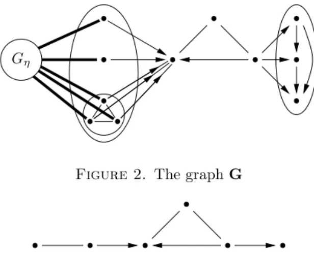
Example 5.1. Consider the graphG of Figure 2. The thick edges stand for all edges between the copy of Gη (from Example 4.4) and their end vertices to the right. The graphG is robust of type (IV). It has a unique prime factor Pshown on Figure 3. It has a unique elementary factor of type (III), and countably many elementary factors of type (I) and (II) (those of the copies ofGη), and it has one
9The linear order on the sons of a node of type III is encoded byf edg. If in this ordering, every element has as successor and a predecessor (unless it is minimal or maximal), it is enough to encode byf edgthe successor of each node.