HAL Id: hal-01346096
https://hal.archives-ouvertes.fr/hal-01346096v2
Submitted on 10 Feb 2017
HAL
is a multi-disciplinary open access archive for the deposit and dissemination of sci- entific research documents, whether they are pub- lished or not. The documents may come from teaching and research institutions in France or abroad, or from public or private research centers.
L’archive ouverte pluridisciplinaire
HAL, estdestinée au dépôt et à la diffusion de documents scientifiques de niveau recherche, publiés ou non, émanant des établissements d’enseignement et de recherche français ou étrangers, des laboratoires publics ou privés.
Numerical modeling of three-dimensional open elastic waveguides combining semi-analytical finite element and
perflectly matched layer methods
Khac-Long Nguyen, Fabien Treyssede, Christophe Hazard
To cite this version:
Khac-Long Nguyen, Fabien Treyssede, Christophe Hazard. Numerical modeling of three-dimensional open elastic waveguides combining semi-analytical finite element and perflectly matched layer methods.
Journal of Sound and Vibration, Elsevier, 2015, 344, pp.158-178. �10.1016/j.jsv.2014.12.032�. �hal-
01346096v2�
Numerical modeling of three-dimensional open elastic waveguides combining semi-analytical finite element and perfectly matched layer methods
K. L. Nguyena,∗, F. Treyss`edea, C. Hazardb
aLUNAM Universit´e, IFSTTAR, GERS, F-44344 Bouguenais, France
bENSTA-UMA, POEMS, 828 Boulevard des Mar´echaux, 91120 Palaiseau, France
Abstract
Among the numerous techniques of non destructive evaluation, elastic guided waves are of particular interest to evaluate defects inside industrial and civil elongated structures owing to their ability to propagate over long distances. However for guiding structures buried in large solid media, waves can be strongly attenuated along the guide axis due to the energy radiation into the surrounding medium, usually considered as unbounded. Hence, searching the less attenuated modes become necessary in order to maximize the inspection distance. In the numerical modeling of embedded waveguides, the main difficulty is to account for the unbounded section. This paper presents a numerical approach combining a semi-analytical finite element method and a perfectly matched layer (PML) technique to compute the so-called trapped and leaky modes in three-dimensional embedded elastic waveguides of arbitrary cross-section. Two kinds of PML, namely the Cartesian PML and the radial PML, are considered. In order to understand the various spectral objects obtained by the method, the PML parameters effects upon the eigenvalue spectrum are highlighted through analytical studies and numerical experiments. Then, dispersion curves are computed for test cases taken from the literature in order to validate the approach.
Keywords:
1. Introduction
Among the numerous techniques of non destructive evaluation (NDE), elastic guided waves are of particular interest to evaluate defects inside industrial and civil elongated structures due to their ability to propagate over long distances. Two categories of waveguides can be distinguished: closed waveguides (guides in vacuum) and open waveguides (embedded waveguides).
In closed waveguides, waves can propagate along the guide axis without attenuation. However in practice, guides are often embedded in large solid media that can be considered as unbounded. In this case, waveguides are called open because of the energy radiation into the surrounding medium. Three kinds of wave modes can occur in open waveguides: radiation modes, trapped modes and leaky ones. Their characteristics are briefly recalled in the following paragraphs. These modes are obtained by assuming a dependence of wave fields in ei(kz−ωt), where k is the axial wavenumber,ωis the angular frequency and z is the coordinate along the waveguide axis. The following dispersion relations holds: k2+k2l/s=ω2/c2l/s, where cland csare the longitudinal and shear wave speeds, kland ksdenote the longitudinal and shear transverse wavenumbers of the unbounded medium respectively.
Radiation modes are standing waves in the transverse directions and can be either oscillating or evanescent in the longitudinal direction, i.e. kl/s∈Rand k is real or pure imaginary. They constitute a continuous spectrum [1, 2], resulting from the unbounded nature of the problem. Resonating mainly in the surrounding medium, radiation modes are of little interest for the NDE of elongated structures.
Conversely, trapped modes are of particular interest. These modes exponentially decay in the transverse di- rections (kl/s∈iR) and propagate along the axis without attenuation (k∈R) in non-dissipative waveguides. Their
∗Corresponding author
Email address:khac-long.nguyen@ifsttar.fr(K. L. Nguyen)
Preprint submitted to Journal of Sound and Vibration November 23, 2014
NGUYEN, Khac-long, TREYSSEDE, Fabien, HAZARD, Christophe, 2015, Numerical modeling of three-dimensional open elastic waveguides combining semi-analytical finite element and perflectly matched layer methods, Journal of Sound and Vibration, Elsevier, 344, pp.158-178, DOI: 10.1016/j.jsv.2014.12.032
energy is confined into the core of waveguides without energy leakage into the surrounding medium allowing long inspection distances. Nevertheless, trapped modes do not always occur. For scalar open waveguides (char- acterized by a scalar field such as the acoustic pressure or the SH wave displacement), trapped modes exist only if the bulk velocity in the core is lower than in the surrounding medium [3]. In the elastic case, both compressional and shear bulk waves occur and, unless Stoneley waves are allowed on the interface between materials, no trapped modes are present when the shear velocity is faster in the core [4, 5]. Unfortunately, such a configuration is often encountered in civil structures because the guiding structures are usually embedded in soft solid media such as concrete, cement or grout for instance.
As opposed to trapped modes, leaky modes always exist in open waveguides. Their energy leakage into the surrounding medium yields attenuation along the guide axis (k ∈ C/R, Im(k) being positive for positive- going modes and negative for negative-going ones), which can strongly limit their propagation distance. An unusual behavior of leaky modes is that, while decaying along the axis, their amplitudes increase in the trans- verse directions. This feature is well-known in electromagnetism [3, 6] and has sometimes been mentioned in elastodynamics [7, 8, 9, 10, 11].
From a mathematical point of view, leaky modes are not spectral objects because they belong to the forbidden Riemann sheet [3, 12]. They constitute a discrete set which is not part of the complete set constituted by the continuum of radiation modes and the discrete set of trapped modes [1, 2]. The mathematical characterization of leaky modes requires a complicated analytical continuation [13] which is out of scope here. From a physical point of view, leaky modes can constitute a good approximation of the continuum of radiation modes in the excited field over a restricted area, near the core region [6]. Through the imaginary part of their axial wavenumbers, leaky modes allow to directly evaluate the ability of waves to propagate far away along the axis. With radiation modes, such an information is hidden into the continuum. Therefore, an accurate determination of leaky modes is essential for the NDE of embedded waveguides in order to find modes and frequencies of lowest attenuation.
In the literature, many researches have been conducted on embedded waveguides based on analytical ap- proaches [14, 15]. Analytical models are mainly based on transfer matrix or global matrix methods [14, 15] and allow to plot the dispersion curves of solid embedded waveguides. Methods based on Debye series have also been proposed in Ref. [16]. Yet, these techniques are limited to simple geometries such as plates and cylin- ders [17, 18, 19].
The modeling of more complex geometries usually relies on numerical approaches. A powerful technique is the so-called Semi-Analytical Finite Element (SAFE) method [20, 21, 22, 23], which restricts the FE dis- cretization on transverse directions only. The SAFE method has been mainly used for the simulation of closed waveguides. The numerical modeling of open waveguides encounters two difficulties: the cross-section is un- bounded and the amplitude of leaky modes transversely increases. In order to overcome these difficulties, the SAFE method must be associated with other techniques.
A simple numerical procedure is the absorbing layer (AL) method proposed in Refs. [24, 25], which consists in creating artificial viscoelastic layers in the surrounding medium for absorbing waves. Instead of using artificial layers, Mazzotti et al. have recently combined the boundary element method (BEM) with the SAFE method to model three-dimensional elastic waveguides embedded in a solid [26] or in a fluid [27]. The BEM expresses the solution in the exterior domain by integral formula on the core boundary. Analogously to the SAFE-BEM method, Hayashi et al. [28] have proposed a formulation for open plate waveguides. An alternative technique is the perfectly matched layer (PML) method, which consists in analytically extending real coordinates of physical equations into the complex ones. The SAFE-PML method has already been applied to scalar wave problems [29, 30, 31]. More recently, the authors have presented this method to model open solid plate waveguides [32, 33]
(one-dimensional modal problems).
Among these three techniques, the SAFE-AL method is the simplest to implement as it does not require spe- cific programming in existing codes. However, the AL artificial viscoelasticity must be slowly growing in order to minimize reflection so that large layers can be required in practice, hence increasing the computational cost.
Compared to AL, the PML thickness is expected to be significantly reduced. Theoretically, the PML can strongly attenuate waves without artificial reflection thanks to the analytical extension of coordinates (perfectly matched property). Contrary to SAFE-AL and SAFE-PML methods, the SAFE-BEM method avoids the discretization of the unbounded medium, which significantly reduces the computational domain. Yet, the SAFE-BEM eigen- problem is highly non linear and difficult to solve. To avoid the eigenproblem non-linearity with SAFE-BEM
2
(a) (b) (c)
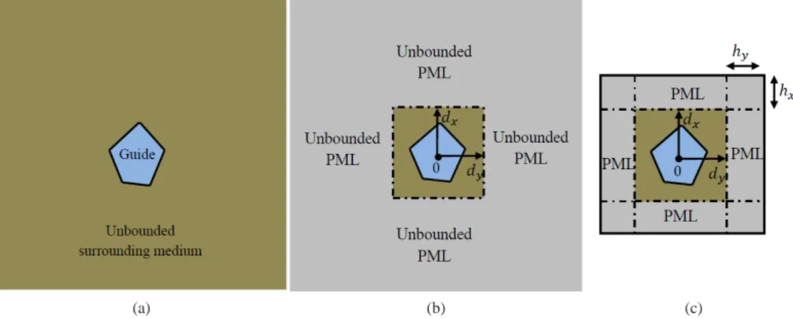
Figure 1: (a) Arbitrary cross-section of an open waveguide, (b) introduction of Cartesian PML in the surrounding medium, (c) PML truncation.
methods, some modified formulations have been proposed. Hayashi et al. [28] have successfully transformed the non linear eigenproblem into a linear one for the special case of a surrounding fluid (scalar waves). Gravenkamp et al. [34] have proposed a simplified boundary condition, namely dashpot boundary condition, which amounts to neglect transverse wavenumbers in the exact radiation condition. This dashpot condition is usually no longer accurate for low frequency or for low contrast of acoustic impedance. Unlike the SAFE-BEM approach, both the SAFE-AL and SAFE-PML methods yield a linear eigenvalue problem.
In this paper, the SAFE-PML technique is proposed as an alternative to SAFE-AL and SAFE-BEM methods to compute modes in three-dimensional elastic waveguides of arbitrary cross-section embedded in an unbounded solid matrix. Two kinds of PML, Cartesian and radial, are considered. This yields two formulations referred to as the SAFE-Cartesian PML (SAFE-CPML) method and the SAFE-radial PML (SAFE-RPML) method. It is pointed out that both kinds of PML have been analyzed mathematically for computing the acoustic resonances of open cavities [35, 36], which constitutes a problem close to that of the present paper. Note also that the SAFE- CPML formulation of this paper is indeed similar to the 2.5D displacement-based PML formulation recently proposed in Ref. [37] (yet in this reference, the discretized problem was not considered as an eigenvalue problem, but rather inverted by considering a source term for fixed transverse wavenumbers).
This paper focuses on the implementation and the validation of the SAFE-PML method. The comparative study between this technique and other techniques such as SAFE-AL or SAFE-BEM methods is out of scope of this paper and left for further studies.
The SAFE-CPML and SAFE-RPML formulations are presented in Secs. 2 and 3 respectively. In order to understand the various spectral objects obtained from these formulations and to clarify the effects of PML parameters, the eigenvalue spectrum is analyzed for each formulation based on analytical studies and numerical experiments. In Sec. 4, the computation of modal properties (group velocity, energy velocity and kinetic energy) is introduced and dispersion curves are computed for several test cases taken from the literature to validate both formulations.
2. SAFE - CPML method
2.1. Initial formulation of 3D elastodynamics
One considers a three-dimensional waveguide ˜Ω =S˜×]− ∞,+∞[. Linear elastic materials are assumed. The waveguide cross-section ˜S lies in the ( ˜x,˜y) plane. The tilde notation will be explained through the introduction of PML in Sec. 2.2. The time harmonic dependence is chosen as e−iωt. The study is focused on eigenmodes.
Acoustic sources and external forces are then discarded.
The variational formulation of the elastodynamic problem for the displacement field u is given by Z
Ω˜
δ˜ǫTσd ˜˜ Ω−ω2 Z
Ω˜
ρδ˜u˜ T˜ud ˜Ω =0 (1)
3
where d ˜Ω =d ˜xd˜ydz. This formulation holds for any kinematically admissible displacementδ˜u=[δ˜uxδ˜uyδ˜uz]T. The notationδ˜ǫ =[δǫ˜xxδ˜ǫyy δ˜ǫzz2δ˜ǫxy2δ˜ǫxz2δǫyz]T is the virtual strain vector, ˜σ =[ ˜σxxσ˜yyσ˜zz σ˜xy σ˜xzσ˜yz]T denotes the stress vector. The stress-strain relation is given by ˜σ = C˜˜ǫ, where ˜C is the matrix of material properties. ˜ρis the material mass density. The superscript T denotes the matrix transpose. We assume that ˜C and ˜ρdepend only on the transverse coordinates ( ˜x,˜y), which means that we consider translationally invariant waveguides along the z axis. Moreover we assume that the medium is homogeneous outside a bounded region which represents the core of the waveguide.
Separating transverse from axial derivatives, the strain-displacement relation can be written as follows:
˜
ǫ= LS˜ +Lz
∂
∂z
!
˜u (2)
where LS˜ =Lx
∂
∂˜x +Ly
∂
∂˜yand
Lx=
1 0 0
0 0 0
0 0 0
0 1 0
0 0 1
0 0 0
, Ly=
0 0 0
0 1 0
0 0 0
1 0 0
0 0 0
0 0 1
, Lz=
0 0 0
0 0 0
0 0 1
0 0 0
1 0 0
0 1 0
. (3)
LS˜ and Lz∂/∂z are the operators of derivatives with respect to the transverse directions ( ˜x,˜y) and the axis z respectively.
2.2. Combining SAFE and Cartesian PML techniques
The SAFE method consists in assuming a harmonic axial dependence of fields and applying the FE method to the transverse directions. The problem is then reduced from three dimensions to the two dimensions of the waveguide cross-section. The SAFE method has been widely used for modeling closed waveguides (guides in vacuum), for which the cross-section is bounded (see for instance [20, 21, 22, 23]).
The modeling of open waveguides requires to combine the SAFE method with another technique due to the unbounded nature of the section. We assume that outside a possibly inhomogeneous region representing the core of the waveguide, the medium is homogeneous. The basic idea consists in closing the waveguide section by replacing the unbounded homogeneous region with a PML of finite thickness. As shown in Fig. 1, a PML is introduced along the Cartesian transverse coordinates in order to attenuate waves in the surrounding medium. By truncating the cross-section to a sufficiently large distance, the problem becomes closed and the SAFE method can be applied. In this case, ˜S denotes the truncated section including the PML.
The basic principle of PML can be readily understood in a one-dimensional situation. Consider for instance the case of a longitudinal wave traveling in the positive ˜x direction. Such a wave can be expressed as an ex- ponential function exp(ikl˜x), which extends to an entire function for complex values of ˜x. Hence, instead of considering real ˜x, one can choose a particular path ˜x(x) in the complex plane parametrized by a real variable x such that exp(ikl˜x(x)) decays exponentially as x tends to+∞. The same considerations apply in the ˜y direction or for a shear wave. The Cartesian PML method consists in extending the initial equilibrium equations to complex coordinates ˜x and ˜y, properly parametrized to attenuate waves (the PML parametrization will be discussed in Sec. 2.4). Here we define
˜x(x)= Z x
0
γx(ξ)dξ, ˜y(y)= Z y
0
γy(ξ)dξ (4)
whereγx(x),γy(y) are complex functions satisfying
• γx(x)=1 for|x| ≤dx;γy(y)=1 for|y| ≤dy,
• Im{γx}>0 for|x|>dx; Im{γy}>0 for|y|>dy. 4
dxand dyare positive parameters chosen such that the rectangle [−dx,+dx]×[−dy,+dy] contains the inhomoge- neous part of the medium. Thus ˜x and ˜y become non-real in the homogeneous surrounding medium.
Since waves are attenuated, the PML can be truncated at a finite distance. We denote by hxand hythe PML thicknesses in the x and y directions respectively (see Fig. 1c). Thus, in the (x,y) plane, the truncated cross-section including the PML is the rectangle of half-thicknesses dx+hxand dy+hy. On the exterior boundary of the PML, the boundary condition can be arbitrarily chosen (usually of Dirichlet type).
From Eq. (4), the change of variables ˜x7→x, ˜y7→y yields for any function ˜f :
∂f˜
∂˜x = 1 γx
∂f
∂x, ∂f˜
∂˜y = 1 γy
∂f
∂y, d ˜x=γxdx, d˜y=γydy (5) where ˜f ( ˜x(x),˜y(y),z)= f (x,y,z).
Applying this change of variable to Eq. (2) leaves the operator Lzunchanged while the operator LS˜ has to be replaced with
LS = 1 γxLx ∂
∂x+ 1 γyLy∂
∂y. (6)
Now applying the SAFE method, the displacement u and the virtual displacementδu are expressed on one element e as follows:
u(x,y,z)=Ne(x,y)Ueeikz, δu(x,y,z)=Ne(x,y)δUee-ikz (7) where k is the axial wavenumber, Ueis the displacement vector and Neis the matrix of interpolating functions on the element e.
Replacing the axial derivative∂/∂z of the trial and test functions with products by+ik and−ik respectively, the formulation (1) is reduced from three dimensions (x,y,z) to a bidimensional problem written in the transverse directions (x,y). The strain-displacement relation becomes
ǫ =(LS +ikLz) NeUeeikz. (8) The FE discretization of the truncated cross-section finally yields
{K1−ω2M+ik(K2−KT2)+k2K3}U=0 (9) with the elementary matrices:
Ke1= Z
e
NeTLTSCLSNeγxγydxdy,Ke2= Z
e
NeTLTSCLzNeγxγydxdy Ke3=
Z
e
NeTLTzCLzNeγxγydxdy,Me= Z
e
ρNeTNeγxγydxdy.
Note that the SAFE-CPML matrices are complex due to the functionsγxandγyin the integrands.
2.3. Linear eigenvalue problem
Given the frequencyω, the formulation (9) is quadratic with respect to k, which can be linearized as [33, 38]
(A−kB) ˆU=0 (10)
with
A=
"
0 I
−(K1−ω2M) −i(K2−KT2)
# , B=
"
I 0 0 K3
# , Uˆ =
"
U kU
#
. (11)
The symmetry of K1, K3 and M implies that if k is an eigenvalue of (9), then−k is also an eigenvalue.
Thus, the eigenspectrum includes two families of solutions, (kj,U+j) and (−kj,U−j), ( j=1, . . . ,n) representing n positive-going and n negative-going waves.
In the presence of PML, K1, K2, K3 and M are complex. A and B are not Hermitian, which somewhat complicates the numerical treatment of the eigensystem (10). As outlined in Ref. [35, 30], the non-hermitian character of matrices may yield spurious eigenvalues which are associated with large values of the norm of resolvent. This problem can be reduced by setting the PML not too far from the core.
In this paper, the ARPACK library [39] is used for solving the eigensystem (10). This library is based on the implicitly restarted Arnoldi method. For each frequency, a specified number of eigenvalues is looked for around a user-defined shift.
5
2.4. PML absorbing functions
In each direction x and y, the PML depends on three user-defined parameters: the position of the interface (dx,dy), the thickness (hx,hy) and the absorbing function (γx,γy). For a given interface position and PML thick- ness, the optimal choice of absorbing functions is crucial for maximizing the attenuation of waves with minimal reflections.
In scattering problems (source problems), the PML function is usually frequency dependent [40, 41] and chosen as:γx(x)=1+iσx(x)/ωwhereσx(x) is a continuous function, parabolic inside the PML region (a similar expression holds forγy(y)). In modal problems, the proper choice of PML functions is slightly different.
As mentioned in the preceding section, if we consider a longitudinal or shear wave exp(ikl/s˜x) for real ˜x (where kland ksdenote the transverse longitudinal and shear wavenumbers), the effect of an infinite PML in the positive x direction is to transform this function into an exponentially decaying function exp(ikl/s˜x(x)) as x tends to+∞. From (4), it is easily seen that the total attenuation across a layer of finite thickness hxis given by
exp(−Im(kl/sγˆxhx))=exp(−|kl/s||γˆx|hxsin(arg kl/s+arg ˆγx)) (12) where ˆγxdenotes the average values ofγxin the layer :
ˆ γx= 1
hx
Z dx+hx dx
γx(ξ)dξ. (13)
One recalls that leaky modes decay along the axial direction z (Im k>0) but grow in the transverse direction, i.e. Im kl/s<0 or equivalently arg kl/s<0. From Eq. (12), leaky waves can be attenuated by the PML if ˆγxis such that arg kl/s>−arg ˆγx(in this paper, arg denotes the principal argument and lies in the interval ]−π,+π]). Hence, increasing arg ˆγxwill enlarge the region of the complex plane where leaky modes can be computed. Increasing
|γˆx|hxwill increase the PML absorption.
For trapped modes, waves propagate without axial attenuation (Imk = 0) and exponentially decay in the transverse direction so that: Rekl/s =0 and Imkl/s >0, or equivalently arg kl/s =π/2. In the presence of PML, trapped waves will thus remain decaying if arg ˆγx < π/2. The PML will be able to enhance the natural decay of trapped modes if Im(kl/sγˆx)>Im kl/s, or equivalently Re ˆγx>1.
Note that|γˆx|cannot be too high in practice for a given hx, otherwise waves will attenuate too fast to be well approximated by the FE discretization. This phenomenon is well-known in the PML literature [40].
For a PML introduced in the y-direction, the above considerations also holds with ˆγydefined by γˆy= 1
hy
Z dy+hy dy
γy(ξ)dξ. (14)
For open waveguide modal problems, the PML functions have been usually set to a constant complex value [30, 42, 43, 44], yielding a discontinuity at the PML interface. However a smooth profile can improve the accuracy of modes, as recently shown in Refs. [32, 33]. In this paper, a parabolic function is set for both the real and the imaginary parts ofγxandγy:
γx(x)=
1 if |x| ≤dx
1+3( ˆγx−1) |x| −dx
hx
!2
if |x|>dx
, γy(y)=
1 if |y| ≤dy
1+3( ˆγy−1) |y| −dy hy
!2
if |y|>dy
. (15)
ˆ
γx and ˆγy quantify the PML absorption. Note that the PML functionsγxandγy are independent ofω, which avoids the calculation of SAFE-CPML matrices at each frequency.
2.5. Eigenspectrum
The goal of this subsection is to get a better understanding of the influence of each PML parameter upon each type of modes. First, the analytical solution of a homogeneous medium is derived and compared with numerical results obtained with the SAFE-CPML method. Second, a more complex case corresponding to a steel cylinder buried in a solid medium is considered. Numerical experiments are performed to understand how the Cartesian PML acts on the eigenspectrum.
6
2.5.1. Homogeneous medium
An isotropic elastic homogeneous medium in three dimensions can be viewed as an open homogeneous waveguide of unbounded section in the (x,y) plane (z being the axial direction). Introducing a PML of finite thickness in both directions x and y, the problem becomes closed. A boundary condition, defined later, must be applied at the PML ends. Let us denoteℓxandℓythe half thicknesses of the whole cross-section (ℓx=dx+hx, ℓy=dy+hy). ˜ℓxand ˜ℓyare the complex half thicknesses, defined as follows:
ℓ˜x= Z ℓx
0
γx(ξ)dξ=dx+γˆxhx, ℓ˜y= Z ℓy
0
γy(ξ)dξ=dy+γˆyhy. (16) Analytical solution. Applying the Helmholtz decomposition [45], the displacement vector ˜u is written as ˜u =
∇˜φ˜+∇ ∧˜ ψ˜(with ˜∇ ·ψ˜ =0), where ˜φand ˜ψ=[ ˜ψx ψ˜y ψ˜z]T are scalar and vector potentials corresponding to lon- gitudinal (l) and shear (s) waves respectively. The equilibrium equations of elastodynamics yield the uncoupled differential equations for potentials:
∂2φ˜
∂˜x2 +∂2φ˜
∂˜y2 +
ω2
c2l +λ
φ˜=0 and ∂2ψ˜
∂˜x2 +∂2ψ˜
∂˜y2 + ω2 c2s +λ
!
ψ˜ =0, (17) whereλ=−k2. cland csare the bulk velocities of longitudinal and shear waves respectively.
Free or Dirichlet boundary conditions couple the potentials ˜φand ˜ψso that fully analytical solutions are not achievable. Instead, the following mixed boundary conditions are considered:
˜ux=0, σ˜xy =0, σ˜xz=0 at ˜x=±ℓ˜x and ˜uy=0, σ˜xy =0, σ˜yz=0 at ˜y=±ℓ˜y. (18) It can be shown that such boundary conditions yield uncoupled boundary conditions for ˜φand ˜ψ:
∂φ˜
∂˜x =0 at ˜x=±ℓ˜x
∂φ˜
∂˜y =0 at ˜y=±ℓ˜y
∂ψ˜x
∂˜x =0 at ˜x=±ℓ˜x
ψ˜x=0 at ˜y=±ℓ˜y
ψ˜y=0 at ˜x=±ℓ˜x
∂ψ˜y
∂˜y =0 at ˜y=±ℓ˜y
ψ˜z=0 at ˜x=±ℓ˜x
ψ˜z=0 at ˜y=±ℓ˜y
. (19)
By separating the variables ˜x and ˜y, the eigenvalues of the problem (17) and (19) are given by λ(p,q)l =−ω2
c2l + pπ 2 ˜ℓx
!2
+
qπ 2 ˜ℓy
2
, λ(m,n)s =−ω2 c2s + mπ
2 ˜ℓx
!2
+
nπ 2 ˜ℓy
2
(20) where m,n,p,q are integers. These apparently formal calculations can be easily justified following the same ideas as in [33].
From Eq. (20), it can be seen that two spectra occur instead of one with scalar waveguides [30, 43]. These two spectra correspond to compressional and shear waves respectively.
Without PML, the eigenvalues are real ( ˜ℓx=ℓx,ℓ˜y=ℓy). In the initial unbounded problem,ℓxandℓytend to infinity: the spectra in terms ofλ=−k2tend to two real continuous half-lines [−ω2/c2l,+∞[ and [−ω2/c2s,+∞[.
These continua of eigenmodes are the so-called radiation modes, which are standing waves oscillating in the transverse directions. As simply shown by Eq. (20), each continuum is discretized by the truncation of cross- section at some finite distance.
With PML, the eigenvaluesλare no longer real. The associated modes are still referred to as radiation modes since they are oscillating inside the PML. In the complexλ-plane, the eigenvalues of Eq. (20) belong to two angular sectors of origins−ω2/c2l and−ω2/c2s. Each sector is limited by two half-lines of rotation angles
−2 arg ˜ℓxand−2 arg ˜ℓy. For clarity, these half-lines are denoted as ∆l/sx
: −ω2/c2l/s+R+/ℓ˜2x,
∆l/sy
: −ω2/c2l/s+R+/ℓ˜2y. (21) Each sector reduces to half-lines if arg ˜ℓx=arg ˜ℓy. When|ℓ˜x|and|ℓ˜y|increase, each spectrum of radiation modes gets denser and becomes continuous when|ℓ˜x|and|ℓ˜y|tend to∞.
7
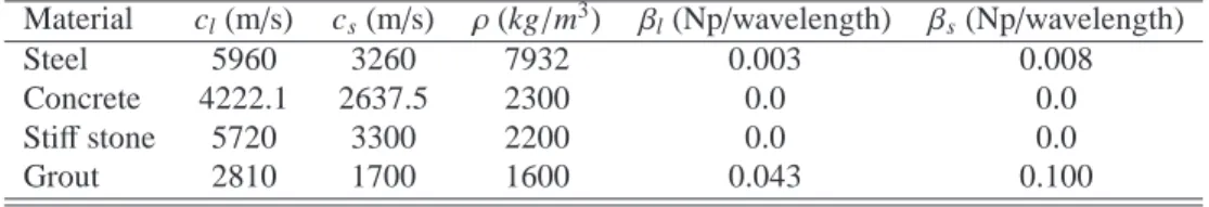
Material cl(m/s) cs(m/s) ρ(kg/m3) βl(Np/wavelength) βs(Np/wavelength)
Steel 5960 3260 7932 0.003 0.008
Concrete 4222.1 2637.5 2300 0.0 0.0
Stiffstone 5720 3300 2200 0.0 0.0
Grout 2810 1700 1600 0.043 0.100
Table 1: Material characteristics.
From Eq. (16), the rotation angles of
∆l/sx and
∆l/sy
are respectively
−2 arg ˜ℓx=−2 arg(dx+γˆxhx), −2 arg ˜ℓy=−2 arg(dy+γˆyhy). (22) This shows that each angle does not depend on the PML function profile itself (only its average value has an effect). It is noteworthy that the result given by Eq. (22) agrees with that obtained in Ref. [46] from a mathematical study of the scalar acoustic PML problem.
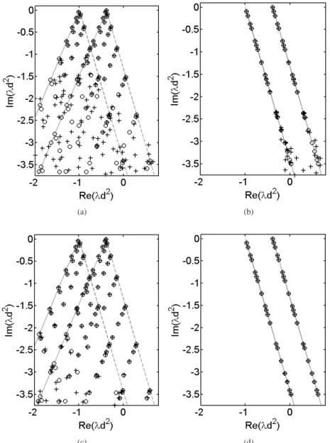
Numerical example. A concrete medium is considered. The material characteristics are given in Tab. 1. The PML interface positions are chosen as dx=dy=d and the PML thicknesses are set to hx=hy=3d. The whole section is a square of half-thicknessesℓx=ℓy=4d.
Figure 2 shows the dimensionless spectrumλd2at the dimensionless angular frequencyΩ =ωd/cs=1 with different values of ˆγxand ˆγy.
As shown in Figs. 2a and 2c, the analytical eigenvalues given by Eq. (20) belong to two angular sectors. They are limited by two half-lines
∆l/sx and
∆l/sy
defined in Eq. (21), rotated from the real axis by angles of−74◦ and−113◦respectively, in agreement with Eq. (22). As can be seen from Figs. 2b and 2d, the angular sectors are reduced to half-lines when PML parameters are identical in both directions.
Numerical eigenvalues computed by the SAFE-CPML method are also shown in Fig. 2 (crosses). The fi- nite elements are six-node triangles, whose average length is denoted by le. The PML functionsγxandγyare parabolic, as defined by Eq. (15).
Numerical results are in agreement with the analytical ones, except for poles that are far from the real axis.
Such poles indeed correspond to higher order modes (higher values of p, q, m, n in Eq. (20)), which have high transverse wavenumbers, i.e. small transverse wavelengths. As in conventional eigenvalue FE problems, these modes are not well approximation due to the FE discretization. Refining the mesh allows to improve numerical results, as confirmed by Figs. 2c and 2d.
2.5.2. Embedded cylindrical elastic waveguides
In this subsection, numerical experiments are conducted on a cylindrical waveguide embedded into a softer solid matrix (the bulk velocities of the core are greater than in the surrounding medium). The test case is taken from the paper of Castaings et al. [24]. It consists of a steel cylinder of 10 mm radius buried in concrete. The material characteristics are given in Tab. 1. The steel is considered as elastic in this test (βl =βs =0, whereβl andβsdenote the longitudinal and shear bulk wave attenuations in Neper per wavelength).
Contrary to the previous subsection, the eigenspectrum now includes leaky modes in addition to radiation modes (note that no trapped modes occur in this test case).
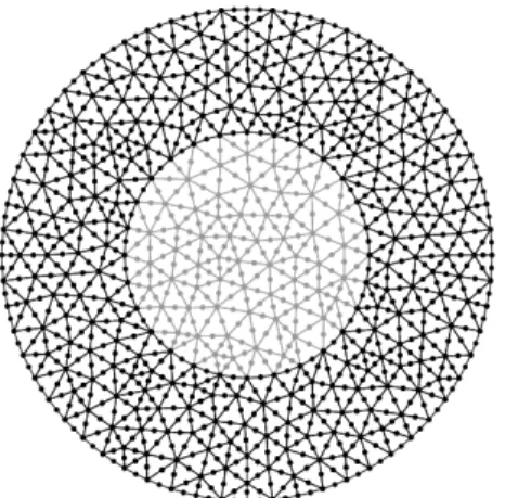
Numerical parameters. The radius of the circular core section is denoted by a. A Dirichlet condition is applied at the exterior boundary of the truncated section. As shown in Fig. 3, finite elements are six-node triangles. PML functions are parabolic. The PML parameters in the x and y directions are identical: dx =dy, hx =hy, ˆγx=γˆy. The PML thicknesses are equal to 0.9a.
Numerical eigenspectrum. Figure 4 represents the dimensionless numerical spectrumλa2 for various PML pa- rameters at the dimensionless frequencyΩ = ωa/cs0 =3.86 (where cs0 is the shear wave velocity of the core).
Two kinds of modes can be distinguished.
8
(a) (b)
(c) (d)
Figure 2: Spectrum of homogeneous concrete medium with section truncated by Cartesian PML atΩ =1 (dx=dy=d, hx=hy=3d) for:
(a) ˆγx=1+i, ˆγy=1+2i, le=0.4d, (b) ˆγx=γˆy=1+i, le=0.4d, (c) ˆγx=1+i, ˆγy=1+2i, le=0.2d and (d) ˆγx=γˆy=1+i, le=0.2d.
Crosses: SAFE-CPML results, circles: analytical results. Dashed lines:
∆l/sx
, continuous lines:
∆l/sy .
9
Figure 3: Cross-section mesh of an embedded cylindrical bar using Cartesian PML (le=0.2a).
(a) (b)
(c) (d)
Figure 4: Numerical spectrum of steel-concrete waveguide obtained atΩ =ωa/cs0=3.86 by the SAFE-CPML method (hx=hy=0.9a) for:
(a) ˆγx=γˆy=2+4i, dx=dy=1.1a, le=0.2a, (b) ˆγx=γˆy=5+4i, dx=dy=1.1a, le=0.2a, (c) ˆγx=γˆy=2+4i, dx=dy=3a, le=0.2a, (d) ˆγx=γˆy=2+4i, dx=dy=1.1a, le=0.1a
10
The first kind corresponds to radiation modes, yielding two spectra of origins (−ω2/c2l,0) and (−ω2/c2s,0), where cl and cs denote the bulk longitudinal and shear wave velocities of the embedding medium (concrete).
Similarly to Sec. 2.5.1, these spectra correspond to the discretized continua of longitudinal and shear waves.
Modes near the origins approximately form straight lines rotated from the real axis with angles equal to 107◦in Fig. 4a and 61◦in Fig. 4b. These angles are in agreement with the analytical formula given by Eq. (22). Far from their origins, radiation modes deviate from straight lines. Such modes are high order modes which the FE mesh can no longer approximate. This is confirmed by Fig. 4d, obtained with a refined mesh (the deviation occurs at a greater distance from the origins).
The rotation of radiation modes indeed allows to discover a second kind of modes, hidden in the original problem without PML. These modes are leaky modes. As observed in Fig. 4, the number of discovered leaky modes grows as the rotation angle is increased: compared to Fig. 4a ( ˆγx=γˆy=2+4i), two leaky modes are not present in Fig. 4b ( ˆγx=γˆy=4+4i). As expected from Sec. 2.4, more leaky modes can be found by increasing the argument of ˆγxand ˆγy.
The rotation angles can also be modified by adjusting the PML interface position dx and dy. Comparing Fig. 4c with 4a shows that high values of dxand dyreduce the rotation angles, in agreement with Eq. (22). In Fig. 4c, note that two leaky modes are spoiled by the deviation of high order radiation modes.
In practice for computing leaky modes, the PML interface should be set close to the core as suggested in Refs. [33, 30, 35]. From a physical point of view, a PML interface too far from the core allows leaky modes to significantly grow before entering the PML, which can deteriorate their computation. This has been mathemati- cally justified by the increase of the norm of the resolvent of the eigenproblem [30, 35].
The spectra of radiation modes can be densified by choosing higher values of PML parameters (dx,dy), (hx,hy) or ( ˆγx,γˆy), which increases the complex half-thicknesses|ℓ˜x|and|ℓ˜y|as explained in Sec. 2.5.1. As an example, compared to Figs. 4a, these spectra get denser in Figs. 4b and 4c, for which the parameters Re ˆγx = Re ˆγyand dx=dyhave been increased respectively.
3. SAFE - RPML method
In this section, the SAFE-RPML formulation is introduced. Following the same approach as in Sec. 2, the associated eigenspectrum is briefly studied through analytical and numerical experiments.
3.1. Combining SAFE and radial PML techniques
The formulation (1) is rewritten in cylindrical coordinates as follows:
Z
Ω˜
δ˜ǫTσ˜rd˜rdθdz˜ −ω2 Z
Ω˜
ρδ˜u˜ T˜u˜rd˜rdθdz=0 (23)
where ˜x=˜r cosθ, ˜y=˜r sinθ. The tilde notation represents the introduction of a PML along the radial direction.
Note that in the above formulation, vectors and tensors are written in cylindrical coordinates but still expressed in the Cartesian basis. In cylindrical coordinates, the operator LS˜ of the strain-displacement relation (2) is
LS˜ =Lx cosθ∂
∂˜r−sinθ
˜r
∂
∂θ
!
+Ly sinθ∂
∂˜r+cosθ
˜r
∂
∂θ
!
. (24)
Applying the PML technique in the radial direction, the formulation (23) can be interpreted as the analytical continuation of the equilibrium equations into the complex radial coordinate ˜r, with
˜r(r)= Z r
0
γ(ξ)dξ (25)
whereγ(r) is a complex function satisfying
• γ(r)=1 for r≤d
• Im{γ}>0 for r>d.
11
Figure 5: Open waveguide with cross-section truncated by radial PML.
d is the position of the PML interface. As shown in Fig. 5, the cross-section of a SAFE-RPML problem is typically a circle of radius d+h, h denoting the PML thickness. Similarly to Cartesian PML, the boundary condition applied at the PML exterior boundary can be arbitrarily chosen.
From Eq. (25), the change of variable ˜r7→r yields for any function ˜f :
∂f˜
∂˜r = 1 γ
∂f
∂r, d˜r=γdr (26)
where ˜f (˜r, θ,z) = f (r, θ,z). Applying this change of variable and the SAFE method to Eqs. (24) leads to an expression identical to Eq. (8), with
LS =Lx
cosθ γ
∂
∂r−sinθ
˜r
∂
∂θ
! +Ly
sinθ γ
∂
∂r+cosθ
˜r
∂
∂θ
!
. (27)
Before FE discretization, the formulation must be transformed back to Cartesian coordinates. The operator LS
then becomes LS =Lx
" x2 γr2 +y2
˜rr
! ∂
∂x+ 1 γr2 − 1
˜rr
! xy ∂
∂y
# +Ly
" 1 γr2 − 1
˜rr
! xy∂
∂x+ y2 γr2 +x2
˜rr
! ∂
∂y
#
. (28)
Finally, the FE discretization of the formulation along the cross-section yields the same form of eigenproblem as Eq. (9), but with the following elementary matrices:
Ke1= Z
e
NeTLTSCLSNe˜rγ
r dxdy,Ke2= Z
e
NeTLTSCLzNe˜rγ r dxdy Ke3=
Z
e
NeTLTzCLzNe˜rγ
r dxdy,Me= Z
e
ρNeTNe˜rγ r dxdy.
3.2. PML absorbing function
As suggested for Cartesian PML, a parabolic profile independent of frequency is chosen for the radial PML functionγ, expressed as follows:
γ(r)=
1 if r≤d
1+3( ˆγ−1) r−d h
!2
if r>d (29)
where ˆγis the average value ofγin the radial PML region:
ˆ γ=1
h Z d+h
d
γ(ξ)dξ (30)
For radial PML, the influence of ˆγon wave absorption can be illustrated by considering wave solutions in cylindrical coordinates. In the PML region (r>d), the wave fields can be expressed by a combination of Hankel
12
functions. Assuming negligible refection from the PML exterior boundary (r=ℓr=d+h), the radial dependence of wave fields is written as Hn(1)(kl/s˜r), where Hn(1)is the Hankel function of first kind and kl/sdenotes the radial wavenumber (shear or longitudinal).
Let us denote the complex radius ˜ℓrby
ℓ˜r= Z ℓr
0
γ(ξ)dξ. (31)
For simplicity, we assume that the radial wavelength is small enough compared to d and|ℓ˜r|(i.e.|kl/sd| ≫1 and
|kl/sℓ˜r| ≫1). Then, the wave solutions at the PML interface and at the PML end, written in terms of H(1)n (kl/sd) and Hn(1)(kl/sℓ˜r) respectively, asymptotically behave like eikl/sd/p
kl/sd and eikl/sℓ˜r/ q
kl/sℓ˜r=
eikl/sd/ q
kl/sℓ˜r
eikl/sγhˆ respectively. Therefore, the total attenuation from the interface to the PML end can then be approximated by
|H(1)n (kl/sℓ˜r)|
|Hn(1)(kl/sd)| ≃exp(−|kl/s||γˆ|h sin(arg kl/s+arg ˆγ)) r
1+γhˆ d
. (32)
Concerning the numerator (exponential term), it can be noticed that the radial wavenumber kl/splays the same role as in Eq. (12). Therefore, the influence of ˆγis similar to the effect of ˆγxand ˆγywith the Cartesian PML method, already described in Sec. 2.4.
The slight difference with radial PML is that this exponential term is modulated by an attenuation factor given by 1/p
|1+γh/dˆ |. Without PML ( ˆγ =1), this attenuation factor corresponds to the geometrical attenuation of cylindrical waves and is equal to 1/√
1+h/d. A radial PML enhances this attenuation factor as|γˆ|increases.
3.3. Eigenspectrum (homogeneous medium)
The SAFE-RPML eigenspectrum is now briefly analyzed in order to understand how a radial PML acts on the eigenspectrum. The analytical solution of a homogeneous medium is derived. Compared to Cartesian coordinates, it is difficult with cylindrical coordinates to find appropriate boundary conditions leading to fully analytical solutions of the elastic problem. Therefore, the analytical solution of this section is obtained for the scalar wave equation of acoustics. The elastic problem will be handled through numerical experiments. For conciseness, this section is limited to the case of a homogeneous medium. The reader is referred to Appendix A for the analysis of a cylindrical core waveguide embedded into an infinite medium, where similarly to the homogeneous case, the analytical solution for an acoustic waveguide is first studied and numerical experiments in the elastic case are then performed.
A homogeneous medium can be considered as an open homogeneous waveguide of unbounded cross-section.
Introducing a radial PML of finite thickness h and of position d, the cross-section becomes bounded and of radius ℓr =d+h.
Analytical solution for a scalar problem. The acoustic wave equation written in cylindrical coordinates is d2φ˜
d˜r2 +1
˜r d ˜φ d˜r −n2
˜r2φ˜+ ω2 c2 −k2
!
φ˜=0 (33)
where ˜φdenotes the acoustic variable, n is the circumferential order and c is the acoustic wave velocity.
The solution of Eq. (33) is ˜φ(˜r) = AJn(kr˜r)+BYn(kr˜r), where kr is the radial wavenumber satisfying the relation kr2+k2 = ω2/c2. Jn and Yn are Bessel functions of the first kind and of the second kind respectively.
Since Yn(kr˜r) tends to infinity when|˜r|tends to 0, B must vanish. A Dirichlet condition ˜φ( ˜ℓr)=0 is applied at the PML exterior boundary, yielding the characteristic equation: Jn(krℓ˜r)=0. The eigenvalues are hence
λnm=−knm2 =−ω2 c2 + χnm
ℓ˜r
!2
(34) whereχnmdenotes the mth zero of Jn(x).
13
Figure 6: Dimensionless spectrum of homogeneous concrete medium computed with the SAFE-RPML method atωd/cs=1. PML parame- ters are h=3d, ˆγ=2+4i (le=0.2d).
Without PML ( ˜ℓr =ℓr), the eigenvalues are real. In the initial problem of infinite section, R tends to infinity and theλspectrum becomes a real continuous half-line [−ω2/c2,+∞[. This continuum can be referred to as the essential spectrum of radiation modes [30, 35].
With a radial PML, the eigenvaluesλof radiation modes become complex. In the complex plane, they belong to a discretized half-line of rotation angle
−2 arg ˜ℓr=−2 arg(d+γh).ˆ (35)
This coincides with the result obtained in Ref. [35] for the computation of acoustic resonances with a radial PML method. Similarly to the Cartesian PML (see Sec. 2.5.1), the discretized half-line gets denser when|ℓ˜r|increases and the rotation angle is independent of the radial PML function profile.
Numerical solution for an elastic problem. The radiation modes of a homogeneous elastic problem are now computed by the SAFE-RPML method. A concrete medium is considered. Finite elements are six-node triangles, whose average length leis chosen as 0.1d. The PML functionγis parabolic, as defined by Eq. (29). The PML thickness is set to h=3d. The radius of the whole cross-section isℓr =4d.
Figure 6 shows the spectrum at the dimensionless frequencyΩ = ωd/cs = 1 with ˆγ = 2+4i. Instead of one half-line with the scalar problem, the eigenvalues belong to two discretized half-lines starting from−ω2/c2l and−ω2/c2s. As already found in Sec. 2.5.1, these two spectra of radiation modes correspond to longitudinal and shear waves respectively (their deviation from straight lines being due to the poor FE approximation of higher order modes).
The half-lines are rotated from the real axis with equal rotation angles, approximately equal to 118◦. This angle is in agreement with the acoustic formula (35).
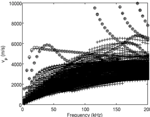
4. Dispersion curves
In this section, the dispersion curves of leaky and trapped modes are computed by both the SAFE-CPML and the SAFE-RPML methods for three test cases taken from the literature. The calculation of modal properties in open waveguides is presented first (kinetic energy, energy velocity and group velocity).
4.1. Kinetic energy
By analytical continuation into complex coordinates, the cross-section and time averaged kinetic energy can be defined as Ek=12R
S˜ ρ˜v˜ ·˜vd ˜S , where ˜v=d ˜u/dt is the velocity vector and bars denote time averaging over one period. As already mentioned in Sec. 2.2, ˜S denotes the waveguide cross-section including the truncated PML.
This definition is rewritten by using the change of variables from complex to real coordinates, as Ek= 1
4 Z
S
ρRe(v∗·v)d ˜S =ω2 4
Z
S
ρRe(u∗· u)d ˜S =ω2 4
Z
S
ρu∗· ud ˜S (36)
14