[PENDING] NUMERICAL SIMULATIONS OF A 2D QUASI GEOSTROPHIC EQUATION

HAL Id: hal-00694541

https://hal.archives-ouvertes.fr/hal-00694541

Submitted on 5 May 2012

HAL is a multi-disciplinary open access archive for the deposit and dissemination of sci- entific research documents, whether they are pub- lished or not. The documents may come from teaching and research institutions in France or abroad, or from public or private research centers.

L’archive ouverte pluridisciplinaire HAL, est destinée au dépôt et à la diffusion de documents scientifiques de niveau recherche, publiés ou non, émanant des établissements d’enseignement et de recherche français ou étrangers, des laboratoires publics ou privés.

NUMERICAL SIMULATIONS OF A 2D QUASI GEOSTROPHIC EQUATION

Jean-Paul Chehab, Maithem Trabelsi Moalla

To cite this version:

Jean-Paul Chehab, Maithem Trabelsi Moalla. NUMERICAL SIMULATIONS OF A 2D QUASI GEOSTROPHIC EQUATION. 2012. �hal-00694541�

NUMERICAL SIMULATIONS OF A 2D QUASI GEOSTROPHIC EQUATION

Jean-Paul Chehab

Laboratoire LAMFA, UMR CNRS 7352 Université de Picardie Jules Verne, Pôle scientifique

33, rue Saint Leu 80037 Amiens cédex, France,jean-paul.chehab@u-picardie.fr

& INRIA Nord-Europe, SIMPAF Project, Villeuneuve d’Ascq, France

Maithem Trabelsi Moalla

Unité de recherche : Multi-Fractals et Ondelettes Faculté des Sciences de Monastir Av. de l’environnement, 5000 Monastir, Tunisie

Abstract

This paper deals with the numerical simulations of the 2D generalized quasi geostrophic equation, where the velocity field is related to the solutionθ by a rotation of Riesz transforms.

Depending on the parameters of the problem, we present numerical evidences for long time behavior of the solution such as global existence effects or blow up in finite time.

1 Introduction

The quasi-geostrophic equations describe large-scale motions in the ocean and atmosphere at middle latitudes. Indeed, air that streams to the south is pushed east or west through Coriolis forces, creating a pressure gradient perpendicular to this motion. The resulting stationary state is called the geostrophic equilibrium. Then, describing the time dependence to lowest order, and since the vertical velocity has to be zero on the bottom of the ocean, or more generally on the lower boundary, the surface behavior can be written independently as a two dimensional equation. This gives rise to the "surface non dissipative quasi-geostrophic equations" see [8].

Here we focus on the 2D dissipative quasi-geostrophic equation, in a generalized version. Let T² be the bi-periodic square[0,1]² ofR², let 0< α ≤1 be fixed and let f ∈L²(T²) be a given scalar time independent function. We are looking for a real scalar functionθ=θ(t, x) defined onR₊×T² representing the temperature of the fluid and satisfying the following dissipative equation:

∂_tθ+ν(−∆)^αθ+u.∇θ=f, x∈T², t >0, (1) and we suppose that the solutionθ satisfies the following initial condition:

θ(0, x) =θ0(x), (2)

whereν> 0 is the viscosity coefficient and u= (u₁, u₂) is the velocity field which is related to the scalarθby a rotation of Riesz transforms:

u = Q_β(−∆)⁻¹²∇^⊥θ, (3)

= Q_β(−∂_x2(−∆)⁻¹²θ, ∂_x1(−∆)⁻¹²θ). (4)

with

Q_β =

µ cosβ −sinβ sinβ cosβ

¶ .

Here β ∈ [0,2π) is a fixed parameter. We mention that when β = kπ we recover the usual 2D dissipative quasi geostrophic equation carrying the name of (SQG), for which the velocity is divergence free, and whenβ6=kπwe recover the generalized 2D quasi geostrophic equation (GSQG).

We notice that we consider periodic boundary conditions onT².

In this paper, we aim at studying numerically the asymptotic behavior of the solutions, associated to both usual and generalized quasi geostrophic equation (SQG) and (GSQG). Part of the numerical simulations are made to confirm the results predicted by the theory, essentially that solutions to (SQG) globally exist for ¹₂ < α≤1,and that solutions to (GSQG) develop finite-time singularities for ¹₄ < α ≤ 1. On the other hand, several numerical tests was performed on a large range of diffusion, viscosity and rotation parametersα, ν and β to depict key parameter dependence of the solutions, and particularly to control the impact of each parameter to guess the blow-up law.

This paper is organized as follows. In the second Section, we introduce the general framework and settings of our study, and we give some list of the existant theory. In section 3, we define the spectral discretization and we propose the numerical time schemes used for the numerical simulations. Then, we discuss their numerical properties in Subsection 3.2.1, namely the mean conservation property, and the numerical stability. Section 4, deals with the numerical simulations for both the usual and the generalized quasi-geostrophic equation.

2 Framework and settings

Before going ahead to exhibit our main results, we shall review the existing dynamic literature.

2.1 The usual quasi geostrophic equation(SQG)

In this section we only focus on the caseβ =kπ, hence we take use of the divergence free property of the velocity field

div u= 0 that is exclusively verified in the non rotational case.

For the (SQG) equation, many studies were concerned with existence and regularity of quasi geostrophic solution, in the continuous case.

Global existence of classical solutions and uniqueness in weaker sense have been resolved for the (SQG) equation in the subcritical caseα > ¹₂, in [9] and [20] for instance. Some global well posedness results are also well known. We refer the reader to [14], [5] and [12] to more details. The critical case α = ¹₂ was first dealt with by Constantin and al in [7] and later studied in [3], [4], [10], [15]

and [26]. The harder case was the supercritical caseα < ¹₂ and it still a big challenge until now.

On the other hand, it is an open problem whether smooth initial data would blow up in finite time. Long time behavior of solutions to the dissipative (SQG) equation with forcing term, has been studied in Berselli [2], where the existence of the global attractor in L² space was proved in the critical caseα= ¹₂, and the existence of the weak global attractor was proved in the subcritical case α ∈ (¹₂,1). Whereas, Ning Ju solves the problem of existence of the global attractor in the

subcritical case with an affirmative answer in [15], see also [21] for a review of fundamental concept and techniques in analysis of infinite dimensional dynamical systems.

From the numerical point of view, Majda and Tabak in [18], first conducted numerical simulations and found that the non dissipative (SQG) equation with smooth initial data develop finite time singularities on∇θ.However a more careful simulation later conducted in [8] and [19] revealed the absence of such singularity and attributed the observation in [18] to a growth of double exponential type.

2.1.1 Analytic properties for (SQG)

We point out that we consider the domain Ω = [0,1]² with periodic boundary conditions. Let us recall Poincaré’s inequality, for any mean zero functionθ:

|(−∆)^α2θ|²2 ≥ C0|θ|²2; (5) ifλ₁ the first nonnegative eigenvalue of the operator(−∆), with periodic boundary conditions, then C₀ =λ^α₁.

Now, the following Lemma is proved.

Lemma 1 We denote by θ¯ = _|Ω|¹ R

Ωθdxdy, the mean of the solution to (SQG), and by f¯ =

1

|Ω|

R

Ωf dxdy, the mean of the external forcef. Then θ¯and f¯satisfy:

1. _dt^dθ¯= ¯f ,

2. if f¯= 0 then θ¯=cte= ¯θ₀,

3. if f = 0 then lim_t→+∞|θ−θ¯|2= 0.

Proof:

1. it is obvious that, since we deal with periodic functions, and using (3) for β =kπ, (−∆)^αθ and ∇(uθ)are mean zero functions, then we get the first property.

2. It follows promptly that if f¯= 0 thenθ¯=cte= ¯θ₀

3. Furthermore, if f = 0 thenθ−θ¯satisfies the following equation:

∂_t(θ) +ν(−∆)^α(θ−θ) +¯ u.∇(θ−θ) = 0,¯ then, taking the inner product withθ−θ, using the relation¯ R

∂tθ(θ−θ)dx¯ =R

∂t(θ−θ)(θ¯ − θ)dx,the Poincaré inequality and the fact that¯ θ−θ¯is mean zero, we obtain:

1 2

d

dt |θ−θ¯|²2 +νC0 |θ−θ¯|²2≤0, hence,

|θ−θ¯|²2≤e^−2νC0t|θ0−θ¯0 |²2 (6) which goes to zero when t goes to infinity.

Concerning the energy point of view, it is well known from the work of S. Resnick [20] that ∀T >

0, θ₀ ∈L², f ∈L¹([0, T], L²) the initial value problem (SQG) admits a solution,

θ∈L^∞([0, T], L²)∩L²([0, T], H^α) (7) that fulfill the energy estimate

|θ(., t)|²2 + Z _t

0 |Λ^αθ(., τ)|²2 dτ ≤|θ(.,0)|²2 + Z _t

0 |f(., τ)|2 dτ, (8) which leads to the energy conservation property in the continuous case whenf = 0.

2.2 The generalized quasi geostrophic equation (GSQG)

In this section we shall focus on the caseβ 6=kπ. Notice that the main problem which leads to the different theoretical study, is the loss of the divergence free property of the velocity field. Indeed, taking the divergence operator of equation (3), one can straightforwardly get

divu= sinβ(−∆)¹²θ

which equals zero only for β = kπ. This lack, ensues automatically the loss of the numerical properties proved for the (SQG) in the sequent section.

Besides, the question of the global well posedness for the (GSQG) was first answered in the super- critical case in [17], the authors restricted their attention to radial solutions of constant sign, and they proved under some conditions on the initial data that the solution blows-up in finite time for 0 ≤α < ¹₄. We notice that they consider the whole domain R² for their analysis and they prove that the blow-up occurs at the level ofk ∇θk∞. However, they mentioned that the restriction of α is just a limitation of their approach and conjectured that singularities exist for all supercritical range0≤α < ¹₂.

It is obvious that radial solutions are steady state solutions for the usual inviscid (SQG) (i.e. ν= 0) which is no longer the case for β 6= kπ. Indeed, Dong and Li proved in [11] that smooth radial solution of the inviscid (GSQG) always develop gradient blow up in finite time. The criteria of blow-up is proved in the whole domainΩ =R² in [17], for the supercritical case, especially in the rangeα ∈(0,¹₄) for smooth radial initial data that satisfies some properties. Besides, Balodis and Còrdoba showed in [1] the existence of singularities for the inviscid (GSQG) equation forβ= ^π₂+kπ.

The authors obtained some new bilinear estimates for the Riesz transforms and used them to show the existence of singularities for general smooth initial data not necessarily radial, and without any restriction on the sign ofθ.

3 Discretization schemes

3.1 Pseudo-spectral space discretization

Due to the periodic boundary conditions, the Fourier pseudo-spectral method appears to be suitable for the space discretization of the problem. We review in this section an essential description of this method, used in our computations.

We recall that for any periodic function f in L²(Ω),f and all their derivatives take an expansion in terms of Fourier series according to:

f(x, y) = X+∞

k1=−∞

X+∞

k2=−∞

f(kˆ ₁, k₂)e^2iπk1.xe^2iπk2.y (9)

where(k₁, k₂) is the fourier discrete vector of Z².

The Fourier coefficientsfˆ(k1, k2)are computed numerically in such a way, that SNf(x, y) interpo- latesf at the grid points(x_k, y_l), where k, l= 0, ..., N −1. They are defined by the relations:

S_Nf(x_k, y_l) =

N

X2

k1=⁻₂^N+1

N

X2

k2=⁻₂^N+1

fˆ(k₁, k₂)e^2iπk1.xke^2iπk2.yl. (10)

Then, using the discrete orthogonality we get inversely:

fˆ(k₁, k₂)) = 4 N²

N

X2

k=⁻₂^N+1

N

X2

l=⁻₂^N+1

f(x_k, y_l)e^−2iπk1.xke^−2iπk2.yl. (11)

The further, serial pseudo-spectral algorithm being computed in practice ,by using fft routines.

Besides, using (11) and denoting byk= (k1, k2), we define the derivative operators as follows:

div(f)(k) =\ ik.fˆ(k) (12)

Λd^γf(k) = |k|^γ fˆ(k), (13) whereΛ = (−∆)^1/2.

3.2 The time marching schemes

For the time discretization, we propose five different schemes that will allow us not only to compare the numerical results for each of them, but also to validate the codes therein at the same time. We cite namely:

• the Forward Euler scheme,

• the linear Backward Euler scheme,

• the Sanz-Serna Cranck-Nickolson scheme,

• the Splitting scheme,

• the Runge-Kutta scheme.

We define hereafter the different schemes, and we review the existant properties therein. We also derive numerical analysis, for each one, namely concerning the mean conservation, and the numerical stability. In Section 4, we validate our results by implementing all these schemes.

3.2.1 The Forward Euler scheme

Letτ >0 be a fixed real, and settⁿ=nτ forn∈N. Then, we recursively construct elementsθⁿ⁺¹ which approchesθ(tⁿ⁺¹) according to the first order convergence scheme:

θⁿ⁺¹−θⁿ

τ +ν(−∆)^αθⁿ⁺¹+uⁿ⁺¹.∇θⁿ⁺¹=f. (14) Whereθ⁰ is an approximation ofθ₀, and

uⁿ⁺¹ =Q_β(−∆)⁻¹²∇^⊥θⁿ⁺¹.

Existence, uniqueness, regularity results have been established in [23] for the infinite dimensional case. In the finite dimensional case an application of the fixed point Browder’ Theorem, gives promptly the wished result. That is in particular, the sequence(θⁿ)_n given by (14) is well defined for alln∈N, see [22] for more details.

We begin by proving the following Proposition, which is a discrete version of Lemma 1:

Proposition 1 θ¯ⁿ and f¯satisfy:

1. θ¯ⁿ=nτf¯+ ¯θ⁰

2. if f¯= 0 then θ¯ⁿ=cte= ¯θ⁰,

3. if f = 0 then lim_n→+∞|θⁿ−θ¯⁰|2= 0.

Proof:

1. equation (14) is written equivalently as follows:

θⁿ⁺¹+τ ν(−∆)^αθⁿ⁺¹+τ∇.(uⁿ⁺¹θⁿ⁺¹) =τ f+θⁿ. (15) Now getting the mean of equation (15), and using the fact that we treat periodic initial data, and that for these data derivatives are periodic and mean zero functions we get

θ¯ⁿ⁺¹ = ¯θ⁰+τf .¯ (16)

Hence recursively we get the wished result.

2. Since f¯= 0 then the second point follows promptly from the first one.

3. If f = 0, thenθⁿ⁺¹−θ¯⁰ satisfies:

(θⁿ⁺¹−θ¯⁰)−(θⁿ−θ¯⁰)

τ +ν(−∆)^α(θⁿ⁺¹−θ¯⁰) +uⁿ⁺¹.∇(θⁿ⁺¹−θ¯⁰) = 0. (17) Then getting the L² inner product of (17) withθⁿ⁺¹−θ¯⁰, and using the Poincaré inequality (5), and the fact that uⁿ⁺¹ is divergence free, we obtain:

< (θⁿ⁺¹−θ¯⁰)−(θⁿ−θ¯⁰)

τ , θⁿ⁺¹−θ¯⁰>+νC₀ |θⁿ⁺¹−θ¯⁰|²2≤0. (18)

Hence, due to the parallelogram identity we get:

1

2(|θⁿ⁺¹−θ¯⁰|²+|θⁿ⁺¹−θⁿ|²) +C₀ντ |θⁿ⁺¹−θ¯⁰ |²≤ 1

2 |θⁿ−θ¯⁰ |² . (19) Then,

|θⁿ⁺¹−θ¯⁰ |²≤ 1

1 + 2C0ντ |θⁿ−θ¯⁰|², (20) and since _1+2C¹

0ντ <1, we obtain the result by a simple induction.

Now, we prove the unconditional stability of (14) in the sequent Proposition:

Proposition 2 The forward Euler scheme (14), is unconditionally stable. Moreover, we have the following estimate:

|θⁿ⁺¹ |²2≤ 1

1 +ντ C₀ |θⁿ|²2+ τ

4νC₀ |f |²2 . (21)

Proof: taking theL² inner product of (14) with θⁿ⁺¹, leads to:

(θⁿ⁺¹−θⁿ, θⁿ⁺¹) + ντ |(−∆)^α2θⁿ⁺¹ |²2 +τ(uⁿ⁺¹.∇θⁿ⁺¹, θⁿ⁺¹) (22)

= (τ f, θⁿ⁺¹).

Then, applying the paralelogram inequality, Poincaré’s inequality (5), and Young’s inequality on (22), we get:

|θⁿ⁺¹−θⁿ|²2 +|θⁿ⁺¹|²2− |θⁿ|²2 +2ντ C₀ |θⁿ⁺¹ |²2≤ τ²

2ε |f |²2 +ε

2 |θⁿ⁺¹|²2, (23) for anyε >0. Now, choosingε= 2ντ C0 ensues:

|θⁿ⁺¹ |²2≤ 1

1 +ντ C₀ |θⁿ|²2+ τ

4νC₀ |f |²2 . (24)

Letγ = _{1+ντ C}¹

0 which is a constant <1, then, by a simple induction on (24) we obtain:

|θⁿ|²2 ≤ γⁿ|θ⁰ |²2 + τ

4νC0(1−γ) |f |²2 (25)

≤ γⁿ|θ⁰ |²2 +1 +γτ C₀

4ν²C₀ |f |²2 . (26)

Hence,|θⁿ|2 is uniformly bounded in L² and (14) is unconditionally stable. We point out that we have used the divergence free property of the velocity field.

3.2.2 The linearized Backward Euler scheme This one, is a linearized Euler scheme which is given by:

θⁿ⁺¹−θⁿ

τ +ν(−∆)^αθⁿ⁺¹+uⁿ.∇θⁿ⁺¹=f. (27) The linear Backward Euler scheme is also a first order convergence scheme. Furthermore, analogous results concerning well posedness and global existence of solution to (27), are proved in [6], starting from an initial dataθ⁰∈H^α.

On the other hand, proving numerical stability and mean conservation properties of proposition 1 for (27) is identically the same task as for (14), owing to the canceling property of the nonlinear term, then it is omitted for conciseness.

3.2.3 The Sanz-Serna Crank-Nicolson scheme

For sake of precision, we implement this second order convergence’ scheme, which reads:

θⁿ⁺¹−θⁿ

τ +ν(−∆)^α(θⁿ⁺¹+θⁿ

2 ) + (uⁿ⁺¹+uⁿ

2 ).∇(θⁿ⁺¹+θⁿ

2 ) =f. (28)

Obviously, this scheme satisfies as well the two first items of Proposition 1. Let us prove the third one. Indeed, sincef = 0,θⁿ⁺¹−θ¯⁰ satisfies:

(θⁿ⁺¹−θ¯⁰) + ( ¯θ⁰−θⁿ)

τ +ν(−∆)^α(θⁿ⁺¹−θ¯⁰+θⁿ−θ¯⁰

2 ) (29)

+(uⁿ⁺¹+uⁿ

2 ).∇((θⁿ⁺¹−θ¯⁰) + (θⁿ−θ¯⁰)

2 ) = 0.

Then, getting the inner product of (29) with(^{θn+1−θ¯0}₂^+θn−θ¯0), we obtain, 1

2τ(|θⁿ⁺¹−θ¯⁰|²2 − |θⁿ−θ¯⁰|²2) +ν

4 |(−∆)^α2(θⁿ⁺¹−θ¯⁰+θⁿ−θ¯⁰)|²2= 0. (30) It follows by Poincaré’s inequality, that

|θⁿ⁺¹−θ¯⁰|²2 +ντ C₀

2 |θⁿ⁺¹−θ¯⁰+θⁿ−θ¯⁰ |²2≤|θⁿ−θ¯⁰ |²2, (31) and this means that (|θⁿ−θ¯⁰ |²2)_n is a decreasing positive sequence, and hence convergent; ∃l ≥ 0/lim_n→+∞|θⁿ−θ¯⁰ |²2=l.

Then, sinceθⁿ=cteis a solution to (28) with zero forcing term, and that for this case l= 0, thus we get,

n→+∞lim |θⁿ−θ¯⁰ |²2= 0,

and the third item of Proposition 1 is hence proved for the Sanz-Serna Crank-Nicolson scheme.

Remark 1 An application of the fixed point Browder’ Theorem in the finite dimensional case, gives as well that the sequence(θⁿ)_n given by (28) is well defined for alln∈N, by replacing only θⁿ⁺¹ by

θⁿ+θⁿ⁺¹

2 ,see [22].

However, it is shown hereafter, that the discretization (28) is not the better one due to his unfor- tunate local stability. Indeed, we only succeed to get a numerical stability in a range[0, T^∗] for a fixedT^∗, given by the next Proposition:

Proposition 3 Forf ∈L²([0, T^∗], L²)the Sanz-Serna scheme (28) isL²-stable in any range[0, T^∗] for fixed T^∗. Indeed

|θⁿ|²2≤|θ⁰|²2 + T^∗

2νC0 |f |²2. (32)

Proof: taking the inner product of (28) with (^θn+1₂^+θn)we get

|θⁿ⁺¹|²2 − |θⁿ|²2+ντ |(−∆)^α2 θⁿ⁺¹+θⁿ 2 |²2≤ 1

2ε |τ f |²2+ε

2 | θⁿ+θⁿ⁺¹

2 |²2. (33) Then using Poincaré’s inequality (5), and forε=ντ C₀, we infer that

|θⁿ⁺¹ |²2 +ντ C₀

2 | θⁿ⁺¹+θⁿ

2 |²2≤|θⁿ|²2+ τ

2νC0 |f |²2 (34)

Now let T^∗ = n₀τ a fixed finite time. Getting the sum Pn0−1

0 of (34), and using the discrete Gronwall lemma we prove that|θⁿ|is uniformly bounded according to theL² norm for any range [0, T^∗], and particularly we have,

|θⁿ|²2+ντ C₀ 2

nX0−1 k=0

| θ^k+1+θ^k

2 |²2 ≤ |θ⁰|²2+τ(n₀−1)

2νC₀ |f |²2 (35)

≤ |θ⁰|²2+ T^∗

2νC₀ |f |²2 . (36)

Notice that comparing (36) and (26) gives an advantage to the forward and the linear backward euler schemes. Whereas, despite his unconditional stability, using the full implicit Euler scheme, one have to solve a large system of nonlinear equations. Then, the linearized scheme seems to be the perfect one at this stage. Hence, to take advantage of the improvement of the convergence order, without falling into numerical instabilities, we introduce the Strang Splitting scheme.

3.2.4 The Splitting scheme

The splitting approximation that we used here, consists on considering the diffusive and the con- vective parts separately, according to a Strang Formula, as follows.

Let us first define the operatorL_t such that the solution of the linear diffusive part,





∂_tθ+ν(−∆)^αθ= 0, θ(0, .) =θ₀(x),

(37) writes

θ(t, x) =L_t.θ₀(x) =e^{−νt(−∆)α}θ₀(x)

Accordingly, we first consider the diffusive part, and we look for a first intermediate half step solution, given by:

θⁿ⁺¹³ =L^τ

2θⁿ. (38)

The second step of the Strang splitting, consists in taking the solutionθⁿ⁺¹³ of the first step as an initial data to a Sanz-Serna Crank Nicolson discretization for the convective part, with a full time stepτ. Namely, we look for a dataθⁿ⁺²³ solution of,

θⁿ⁺²³ −θⁿ⁺¹³

τ + (uⁿ⁺²³ +uⁿ⁺¹³

2 ).∇(θⁿ⁺²³ +θⁿ⁺¹³

2 ) =f. (39)

Finally, the third step reads:

θⁿ⁺¹=L^τ

2θⁿ⁺²³. (40)

Now, since we used a splitting scheme according to a Strang formula, and the corresponding sub- schemes (38)-(40) have all of them a convergence ordern≥2, then the resulting discrete solution is some second order approximation of the solution to the system (1)-(2).

Proposition 4 For the splitting scheme (38)-(40),θ¯ⁿ andf¯satisfy:

1.

θ¯ⁿ=L_nτθ¯⁰+τ Xn k=0

L₍2k+1

2 )τf ,¯ (41)

2. if f¯= 0 then θ¯ⁿ=L_nτθ¯⁰ →0 when n→+∞, 3. if f = 0 then lim_n→+∞|θⁿ−θ¯ⁿ|2= 0.

Proof:

1. from (39) we get ¯

θⁿ⁺²³ = ¯

θⁿ⁺¹³ +τf ,¯ so using (38) and (40) we deduce that, θⁿ⁺¹¯ =L_τθ¯ⁿ+τ L^τ

2

f .¯ (42)

A simple induction on (42) gives the desired relation.

2. If we replace f¯= 0 in (41), we get θ¯ⁿ =L_nτθ¯⁰ which goes to zero when n →+∞, owing to the definition of L.

3. Now, suppose thatf = 0 Eq.(39) rewrites:

(θ^{n+ 23}−L_{( 2}n+1

2 )τθ¯⁰)−(θ^{n+ 13}−L_{( 2}n+1 2 )τθ¯⁰) τ

+(^{un+ 23+u}₂ ^{n+ 13}).∇(^θ

n+ 23−L_{( 2}n+1 2 )τ

θ¯⁰+θ^{n+ 13}−L_{( 2}n+1 2 )τ

θ¯⁰

2 ) = 0 . (43)

Taking the L² inner product of (43) with ^θ

n+ 23−L_{( 2}n+1

2 )τθ¯⁰+θ^{n+ 13}−L_{( 2}n+1 2 )τθ¯⁰

2 ,it follows that:

|θⁿ⁺²³ −L₍2n+1

2 )τθ¯⁰|²2=|θⁿ⁺¹³ −L₍2n+1

2 )τθ¯⁰ |²2 .

Besides, using this relation and (38), (40) we deduce that:

|θⁿ⁺¹−L_(n+1)τθ¯⁰ |2 = |L^τ

2θⁿ⁺²³ −L_(n+1)τθ¯⁰ |2

≤ |L^τ

2 ||θⁿ⁺²³ −L₍2n+1

2 )τθ¯⁰ |2 (44)

≤ |L^τ

2 ||θⁿ⁺¹³ −L₍2n+1

2 )τθ¯⁰ |2 (45)

≤ |L^τ

2 ||L^τ

2θⁿ−L₍2n+1

2 )τθ¯⁰ |2 (46)

≤ |Lτ ||θⁿ−Lnτθ¯⁰|². (47) Hence the result since |L_τ |<1.

Now, concerning the numerical stability point of view, the splitting scheme is unconditionally stable, owing to:

Proposition 5 We suppose that θ satisfies R

Ωθ(t, x)dx= 0,then the splitting scheme (38)-(40) is unconditionally stable. Moreover we have the following estimate:

|θⁿ⁺¹ |2≤δ|θⁿ|2 +τ√

δ |f |2, (48)

whereδ <1 is a contraction constant given in (53).

Proof: getting theL² inner product of (39) byθⁿ⁺²³ +θⁿ⁺¹³ leads to

|θⁿ⁺²³ |²2− |θⁿ⁺¹³ |²2=τ < f, θⁿ⁺²³ +θⁿ⁺¹³ >_L², (49) then by Cauchy Schwarz we get

|θⁿ⁺²³ |2 − |θⁿ⁺¹³ |2≤τ |f |2 . (50) On the other hand, referring to (38) and (40) and using the definition of the operatorL_t, it becomes obvious that to get the uniform bound on|θⁿ⁺¹ |2 we must contract theL² norm of the operator L_t. Indeed

L_t(θ)(x, y) = X

k1,k2∈Z²

θˆ_k1,k2e^{−νtλαk1,k2}e^2iπk1.xe^2iπk2.y,

whereλ_k1,k2 are the eigenvalues of the operator (−∆)^α.Then using the Parseval identity, we get

|L^τ

2θ|²2= X

k1,k2

|θˆ_k1,k2 |² e^{−ντ λαk1,k2}. (51) It follows, that for some mean zero periodic functionθ,(λ_0,0= 0), we obtain:

|L^τ

2θ|²2≤e^{−ντ λα1,0} |θ|²2, (52) whereλ_1,0 is the first nonnegative eigenvalue.

Hence, setting

δ=e^{−ντ λα1,0} <1, (53)

we ensure thatL^τ

2 is a contraction operator, and that

|Lθ|²2≤δ|θ|²2. (54)

Actually, we insert (54) in (38), (40) and then in (50), to get the wished result:

|θⁿ⁺¹ |2≤δ|θⁿ|2 +τ√

δ |f |2,

and then follows promptly the unconditional stability of the splitting scheme.

Remark 2 It would be possible to consider a first order convergence Strang splitting, if we have discretized the first and the third steps of the splitting according to a forward Euler scheme, and the unconditional stability would remain verified. Particularly, we get the following bound:

|θⁿ⁺¹ |²2≤ 1

1 +ντ C₀ |θⁿ|²2+ 2τ

νC₀ |f |²2 .

Remark 3 We emphasize that the solution θⁿ⁺¹ obtained by the four schemes, fulfill the previous numerical properties, only for the usual quasi geostrophic equation (SQG), due to the divergence free velocity field. Furthermore, owing to the linearity of the spectral discretization, the properties proved for the semi-discretization in time, still available for the full one.

In order to get a full discretization of the equation (1), we shall go back to the pseudo- spectral discretization of the previous subsection. For instance, we insert (12) and (13) on (14), and this leads to the full discretized scheme:

θ[ⁿ⁺¹(Id+ντ |k|^2α) = (cθⁿ+τ[

fⁿ⁺¹)−iτ k. \

(uⁿ⁺¹.θⁿ⁺¹). (55) Whereuⁿ⁺¹=F⁻¹(u[ⁿ⁺¹) and

u[ⁿ⁺¹= (−i k₂

|k|

θ[ⁿ⁺¹, i k₁

|k|

θ[ⁿ⁺¹). (56)

Doing the same for the different time schemes introduced in this section, we get three other full discretizations of (1).

3.2.5 The Runge-Kutta scheme

For an accurate simulation of the blow-up in the case of the (GSQG) equation, we considered this third order convergence scheme introduced by Driscoll in [13]. In that paper, the author proposed a composite method in which different integrators are used for different parts of Fourier Space: a standard Runge-Kutta fourth order integrator (RK4) at the lowest wave numbers and stiffly stable, and a linearly implicit third order Runge-Kutta at high wave numbers where the explicit method fails.

Noting byλthe matrix of the linear term which is here the fractional Laplacian, andf(θ(t))is the nonlinear term which is here the convective term, the equation under consideration is then

θ(t) =˙ f(θ(t)) +λθ(t) (57)

The method consists on partition (57) into

θ(t) =˙ f(θ(t), z(t)) +λθ(t) (58)

z(t) =˙ g(θ(t), z(t)). (59)

Then the scheme reads:

K₁ =θⁿ K˜1 =zⁿ

K2 = (1−1

3τ λ)⁻¹(θⁿ+1

2τ f(K1,K˜1) +1 6τ λK1) K˜2=zⁿ+1

2τ g(K1,K˜1), K₃ = (1−τ λ)⁻¹(θⁿ+1

2τ f(K₂,K˜₂) +1

2τ λK₁−τ λK₂) K˜₃=zⁿ+1

2τ g(K₂,K˜₂) K₄ = (1−1

3τ λ)⁻¹(θⁿ+τ f(K₃,K˜₃) + 2 3τ λK₃) K˜₄=zⁿ+τ g(K₃,K˜₃)

θⁿ⁺¹=θⁿ+1

6τ[f(K₁,K˜₁) +f(K₄,K˜₄) +λ(K₁+K₄)]

+1

3τ[f(K₂,K˜₂) +f(K₃,K˜₃) +λ(K₂+K₃)], zⁿ⁺¹=zⁿ+1

6τ[g(K₁,K˜₁) +g(K₄,K˜₄)] + 1

3τ[g(K₂,K˜₂) +g(K₃,K˜₃)]

We emphasize that this method is a third order stable method, and that his constant error is close to the best achievable, and that our choice is essentially made for optimum performance, especially to get the exact blow-up time in the most perfect manner, and that results obtained by the Driscoll scheme, agrees with those obtained by the linear backward Euler one, for instance.

4 Numerical results

4.1 Aims

Our aim in this paper is to capture some theoretical properties, yet proved in previous works, by numerical simulations on (SQG), namely the global existence effect, and theL² norm conservation property forβ =kπ. Then the first part of numerical computations will be devoted to the validation of our codes, by implementing them at the same time, and comparing the results therein.

On the other hand, we aim to explore the (GSQG) equation, particularly, we discuss the formation of singularities atβ 6=kπ, for various values of the diffusion and the viscosity parameters α andν.

Particularly, we intend to study the interaction of these parameters to get a law which controls the blow-up criteria, that will be discussed in the last part of this section.

Besides, we emphasize that our simulations are performed in the torus T², unlike the paper of José and Lie [17], in which the authors considered the whole space R² and this gives us a good opportunity of comparison.

4.2 Numerical simulations for SQG

We choose Matlab r for the implementation of our codes taking advantage of the built-in FFT commands.

Besides, we notice that we used two different methods for the space discretization: the Fourier pseudo-spectral method and the finite differences one (whose results are not reported here), this last one being first used for validating the Fourier code; however, we point out that the use of the finite differences method allows us to explore new frameworks. Indeed, this code is let to later work to get numerical simulation for homogeneous or open boundary conditions. In this paper we, concentrate only on the spectral code.

To validate our codes, three main tests were implemented using the previous discretizations, ac- cording to (14), (28) and (38)-(40) schemes, starting with the initial data:

θ₀(x, y) = sin(2πx) sin(2πy).

At first, let us check the output of our code when computing the approximation of a real function θgiven by:

θ(x, t) = sin(2πx) sin(2πy) exp(sint) =θexact (60) which is a solution of (1) according to the external force

f =F⁻¹(costθˆ+ν |k|^2αθˆ+ exp(sint)u\0.∇θ). (61) Whereu₀ is the velocity field corresponding to θ₀ according to the formula (3) withβ= 0.

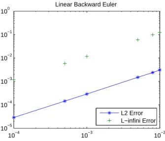
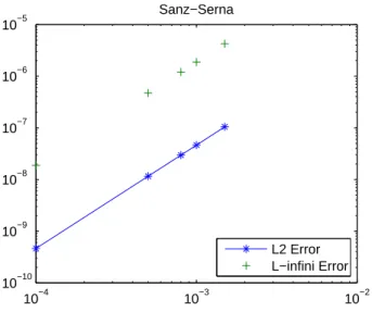
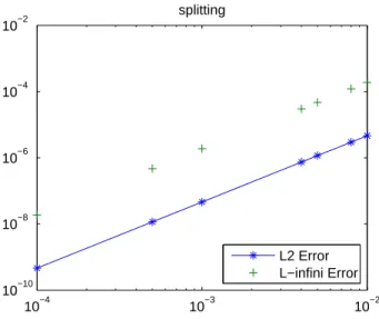
The subsequent figures represent respectively, a mean square fitting of theL²−norm and theL^∞− norm convergence errors. These simulations are results of the forward Euler, the Sanz-Serna and the Splitting schemes with different time steps ∆t. The plots for N = 32, β = 0, ν = 0.0001 and α= 1are given in Figure(1), Figure(2) and Figure(3).

10⁻⁴ 10⁻³ 10⁻² 10⁻⁵

10⁻⁴ 10⁻³ 10⁻² 10⁻¹ 10⁰

Linear Backward Euler

L2 Error L−infini Error

Figure 1: The evolution of the L² error norm and the L^∞ error norm Vs τ for an exact solution according to the linearized backward Euler scheme

10⁻⁴ 10⁻³ 10⁻²

10⁻¹⁰ 10⁻⁹ 10⁻⁸ 10⁻⁷ 10⁻⁶ 10⁻⁵

Sanz−Serna

L2 Error L−infini Error

Figure 2: The evolution of theL² error norm and theL^∞ error norm Vs dτ for an exact solution according to the Sanz-Serna Crank-Nicolson scheme

10⁻⁴ 10⁻³ 10⁻² 10⁻¹⁰

10⁻⁸ 10⁻⁶ 10⁻⁴ 10⁻²

splitting

L2 Error L−infini Error

Figure 3: The evolution of the L² error norm and the L^∞ error norm Vs τ for an exact solution according to the splitting scheme

Hence, we confirm by the previous figures that the error corresponds to a first order convergence scheme, for Figure.(1), and to second order convergence schemes for Figure.(2) and Figure.(3).

Indeed, the slopes of the three curves are given respectively by:

a₁ = 1.036 (62)

a₂ = 2.0018 (63)

a₃ = 2.0015, (64)

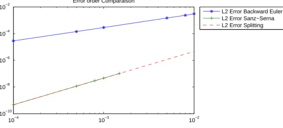
and this contribute to confirm the validity of the codes. Next, we show a comparison between the three curves in Figure (4)

10⁻⁴ 10⁻³ 10⁻²

10⁻¹⁰ 10⁻⁸ 10⁻⁶ 10⁻⁴ 10⁻²

Error order Comparaison

L2 Error Backward Euler L2 Error Sanz−Serna L2 Error Splitting

Figure 4: A comparison between the three schemes of theL² norms Vsτ.

Keeping the same previous parameters α and ν unchanged, we also run numerical simulations of dissipative (SQG) with various initial data and external forces, to display results of proposition 1

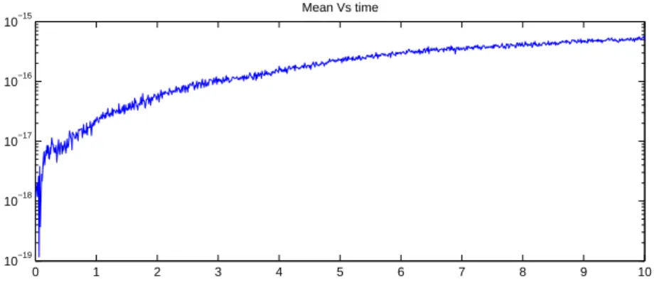
using the linearized backward Euler scheme in Figure(5), the splitting scheme in Figure(6) and the Sanz-Serna scheme in Figure(7). We emphasize that this last test were implemented for ν = 1 for sake of stability. We ran respectively the casesf = 2θ⁰,f = 1andf = 0 emanating from the initial dataθ⁰= sin(2πx) sin(2πy) forN = 64and τ = 10⁻⁴.

0 1 2 3 4 5 6 7 8 9 10

10⁻¹⁹ 10⁻¹⁸ 10⁻¹⁷ 10⁻¹⁶ 10⁻¹⁵

Mean Vs time

Figure 5: The mean of θ Vs time according to the external force f = 2θ0 using the linearized backward Euler scheme

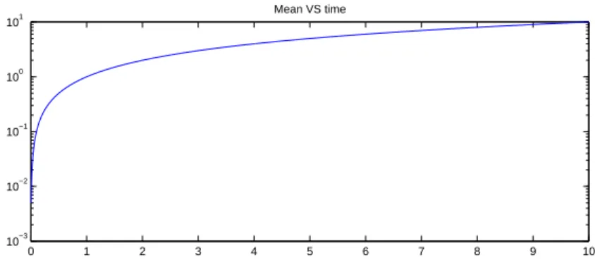
0 1 2 3 4 5 6 7 8 9 10

10⁻³ 10⁻² 10⁻¹ 10⁰ 10¹

Mean VS time

Figure 6: The mean ofθ Vs time according to the external forcef = 1 using the splitting scheme

0 1 2 3 4 5 6 7 8 9 10

10⁻²¹ 10⁻²⁰ 10⁻¹⁹ 10⁻¹⁸

Mean Vs time

Figure 7: The mean of θ Vs time according to the external force f = 0 using the Sanz-Serna Crank-Nicolson scheme

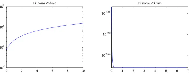
Now we move on towards the third step of validation, to confirm the global existence results of [6]

for instance. For that purpose, we plot the L² norm, and the contour lines of the solution to the dissipative (SQG) for α = 0.67 ≥ ²₃, using the full implicit Euler scheme. By these simulations, we observed that this norm became bounded for t ≥ T^∗ for some fixed time T^∗as illustrated in Figure(8) and Figure(10).

At this point, we underline that for these simulations, we have changed the choice of the initial dataθ⁰ and the external forceF, to restrict ourself only to periodic data that belongs to L² and eventually toL^p for p ≤ _1−α² , and no more regular, to catch exactly results of the main Theorem in [6]. So let θ⁰ = p

sin(2πx(1−x)) sin(2πy(1−y)), and let F = 2θ⁰. The simulations are represented comparatively for the initial and the final step of plotting, in Figure(8) and Figure(9), giving respectively the behavior of the solution, and its contour lines. Whereas in Figure(10) we draw the solution’ L² norm accordingly to F = 2θ⁰ and for F = 0, then the convergence to the global attractor is obviously faster in the second case, owing to the higher regularity of the external force. This is shown in figure (10):

0 50

100 150

0 50 100 150

0 0.5 1 1.5

0 50

100 150

0 50 100 150 15.4 15.45 15.5 15.55 15.6

Figure 8: The evolution of the behavior of anL² initial dataθ⁰, withf = 2θ⁰ according to a full implicit Euler scheme

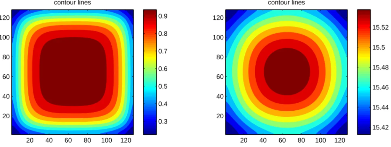
contour lines

20 40 60 80 100 120

20 40 60 80 100 120

0.3 0.4 0.5 0.6 0.7 0.8 0.9

contour lines

20 40 60 80 100 120

20 40 60 80 100 120

15.42 15.44 15.46 15.48 15.5 15.52

Figure 9: The evolution of the contour lines of an L² initial data θ⁰, with f = 2θ0 according to a full implicit Euler scheme.

0 2 4 6 8 10 10⁻¹

10⁰ 10¹ 10²

L2 norm Vs time

0 1 2 3 4 5 6 7

10^−0.21 10^−0.2 10^−0.19

L2 norm VS time

Figure 10: Global existence starting from an L² initial dataθ⁰, first withf = 2θ0 and second forf = 0 according to a full implicit Euler scheme.

Originally, numerical simulations denied the critical behavior atα= ²₃,and even atα= ¹₂.In fact, this can be deduced by the convergence to the global behavior of the discrete solution to the forward Euler scheme atα= ¹₂,in Figure(11).

0

20 40 60 80

0 50

100 15.2 15.4 15.6 15.8

0 2 4 6 8 10

10⁻¹ 10⁰ 10¹ 10²

L2 norm Vs time

contour lines

10 20 30 40 50 60

10 20 30 40 50 60

15.3 15.35 15.4 15.45 15.5

Figure 11: Global existence starting from an L² initial dataθ⁰, withf = 2θ⁰ and α= 0.5 according to a full implicit Euler scheme.

From now on, we focus on the numerical simulations of the generalized quasi-geostrophic equa- tion, forβ∈]0,2π[\kπ. In particular, we aim first to confirm the theoretical predictions of Section 2, and then to catch the real limitation of each parameter to get the blow-up criteria.

4.3 Numerical simulations for (GSQG)

In the sequel, we plot numerical tests, for several values ofα,ν andβ, and the results are illustrated by the next tables. We denote by "Y" the case when the solution blows-up, and by "N" the case when not. We also mention that the tables are arranged in the decreasing order according to the viscosity parameterν which was arbitrary chosen in the set 1, 0.7, 0.5, 0.2,10⁻¹,10⁻²,10⁻³,10⁻⁴. The tables prove the closure interaction between the different parameters, to give the final behavior of the solution.

For these simulations we used the linearized third order Runge-Kutta method given by Driscoll in [13] for the time discretization, and the pseudo-spectral one for the space discretization.

Remark 4 We emphasize that all results obtained according to the Runge-Kutta scheme were al- ready detected for the forward Euler scheme or the Splitting scheme for instance, and that this choice is done only for sake of precision to depict the exact blow-up time.

Remark 5 We restricted our simulations to the range β ∈ [0,^π₂], since we have remarked that blow-up is function ofsinβ, (this will be discussed in details later).

❍❍

❍❍

❍❍ β

α 0.1 0.15 0.2 0.25 0.3 0.35 0.4 0.5 0.8 1

0 N N N N N N N N N N

π

100 N N N N N N N N N N

π

10 N N N N N N N N N N

π

6 N N N N N N N N N N

π

4 Y N N N N N N N N N

π

3 Y N N N N N N N N N

π

2 Y N N N N N N N N N

Table 1: ν = 1, τ = 10⁻⁴

❍❍

❍❍

❍❍ β

α 0.1 0.15 0.2 0.25 0.3 0.35 0.4 0.5 0.8 1

0 N N N N N N N N N N

π

100 N N N N N N N N N N

π

10 N N N N N N N N N N

π

6 N N N N N N N N N N

π

4 Y Y N N N N N N N N

π

3 Y Y N N N N N N N N

π

2 Y Y N N N N N N N N

Table 2: ν= 0.7, τ = 10⁻⁴

❍❍

❍❍

❍❍ β

α 0.1 0.15 0.2 0.25 0.3 0.35 0.4 0.5 0.8 1

0 N N N N N N N N N N

π

100 N N N N N N N N N N

π

10 Y N N N N N N N N N

π

6 Y Y N N N N N N N N

π

4 Y Y N N N N N N N N

π

3 Y Y Y N N N N N N N

π

2 Y Y Y N N N N N N N

Table 3: ν= 0.5, τ = 10⁻⁴

❍❍

❍❍

❍❍ β

α 0.1 0.15 0.2 0.25 0.3 0.35 0.4 0.5 0.8 1

0 N N N N N N N N N N

π

100 N N N N N N N N N N

π

10 Y Y Y Y Y N N N N N

π

6 Y Y Y Y Y N N N N N

π

4 Y Y Y Y Y N N N N N

π

3 Y Y Y Y Y N N N N N

π

2 Y Y Y Y Y N N N N N

Table 4: ν= 0.2, τ = 10⁻⁴

❍

❍❍

❍❍❍ β

α 0.1 0.15 0.2 0.25 0.3 0.35 0.4 0.5 0.8 1

0 N N N N N N N N N N

π

100 N N N N N N N N N N

π

10 Y Y Y Y Y Y N N N N

π

6 Y Y Y Y Y Y N N N N

π

4 Y Y Y Y Y Y N N N N

π

3 Y Y Y Y Y Y N N N N

π

2 Y Y Y Y Y Y N N N N

Table 5: ν = 10⁻¹, τ = 10⁻³

❍❍

❍❍

❍❍ β

α 0.1 0.15 0.2 0.25 0.3 0.35 0.4 0.5 0.6 0.7 0.8 1

0 N N N N N N N N N N N N

π

100 N N N N N N N N N N N N

π

10 Y Y Y Y Y Y Y Y N N N N

π

6 Y Y Y Y Y Y Y Y Y N N N

π

4 Y Y Y Y Y Y Y Y Y N N N

π

3 Y Y Y Y Y Y Y Y Y N N N

π

2 Y Y Y Y Y Y Y Y N N N N

Table 6: ν = 10⁻², τ = 10⁻⁴

The criteria of blow-up detected for example for the caseβ = ^π₃, α= 0.5andν = 10⁻²is illustrated by the following figures which represents the solution’ blow-up and the correspondingL² norm:

0

50

100 150

0 50 100 150

−200

−100 0 100

0 0.1 0.2 0.3 0.4 0.5

10⁰

L2 norm of the solution vs time

Figure 12: resolution with a third order Runge-Kutta scheme. α = 0.5, ν = 10⁻², β = ^π₃, dx = dy= ₁₂₈¹ ,τ = 0.0001;θ⁰= sin(2πx) sin(2πy) andf = 2θ⁰

In [17], Dong Lie and José Rodrigo, have considered the blow-up in the supercritical range, we propose here to complete the study by considering the dissipative parameter α belonging in the whole interval]0,1[; the angleβ ∈[0 +δ, π−δ], where ₁₀₀^π ≤δ ≤ 10^π. We emphasize that we have detected a criteria of blow up for β = ₁₀₀^π , for ν ≤ 10⁻³. This can be observed in the following table: