HAL Id: hal-00546961
https://hal-brgm.archives-ouvertes.fr/hal-00546961
Submitted on 15 Dec 2010
HAL is a multi-disciplinary open access archive for the deposit and dissemination of sci- entific research documents, whether they are pub- lished or not. The documents may come from teaching and research institutions in France or abroad, or from public or private research centers.
L’archive ouverte pluridisciplinaire HAL, est destinée au dépôt et à la diffusion de documents scientifiques de niveau recherche, publiés ou non, émanant des établissements d’enseignement et de recherche français ou étrangers, des laboratoires publics ou privés.
Numerical Simulations of the Thermal Impact of Supercritical CO2 Injection on Chemical Reactivity in a
Carbonate Saline Reservoir
Laurent André, Mohamed Azaroual, André Menjoz
To cite this version:
Laurent André, Mohamed Azaroual, André Menjoz. Numerical Simulations of the Thermal Impact of Supercritical CO2 Injection on Chemical Reactivity in a Carbonate Saline Reservoir. Transport in Porous Media, Springer Verlag, 2010, 82 (1), p. 247-274. �10.1007/s11242-009-9474-2�. �hal-00546961�
Numerical simulations of the thermal impact of supercritical CO
2injection on chemical reactivity in a carbonate saline reservoir
Laurent André, Mohamed Azaroual, André Menjoz
BRGM – Water Division - 3 Avenue Claude Guillemin, BP 36009, F-45060 ORLEANS Cedex 2, France
Tel : +33 (0)2 38 64 31 68 Fax : +33 (0)2 38 64 37 19 Email : l.andre@brgm.fr www.brgm.fr
Abstract Geological sequestration of CO2 offers a promising solution for reducing net emissions of greenhouse gases into the atmosphere. This emerging technology must make it possible to inject CO2 into deep saline aquifers or oil- and gas-depleted reservoirs in the
supercritical state (P > 7.4 MPa and T > 31.1 °C) in order to achieve a higher density and therefore occupy less volume underground. Previous experimental and numerical simulations have
demonstrated that massive CO2 injection in saline reservoirs causes a major disequilibrium of the physical and geochemical characteristics of the host aquifer. The near-well injection zone seems to constitute an underground hydrogeological system particularly impacted by supercritical CO2
injection and the most sensitive area, where chemical phenomena (e.g., mineral
dissolution/precipitation) can have a major impact on the porosity and permeability. Furthermore, these phenomena are highly sensitive to temperature. This study, based on numerical multi-phase simulations, investigates thermal effects during CO2 injection into a deep carbonate formation.
Different thermal processes and their influence on the chemical and mineral reactivity of the saline reservoir are discussed. This study underlines both the minor effects of intrinsic thermal and thermodynamic processes on mineral reactivity in carbonate aquifers, and the influence of anthropic thermal processes (e.g., injection temperature) on the carbonates’ behaviour.
Keywords: coupled modelling, supercritical CO2, saline reservoir, Joule- Thomson effect, geochemical reactivity
1 Introduction
CO2 storage in saline reservoirs is a promising alternative for the sequestration of this greenhouse gas because of their capacity worldwide (Bachu 2002; IPCC 2005). Results of modelling studies suggest that under favourable conditions CO2
can be safety confined for thousands of years (Weir et al. 1996a,b; White et al.
2005). However, before effective and safety containment can be ensured in a selected aquifer, investigations need to be carried out on reservoir behaviour when subjected to physical, chemical, and thermal perturbations induced by massive CO2 injection. If laboratory or field experiments can bring many details about gas behaviour in targeted reservoirs, numerical simulations constitute an integrative tool of main importance to assess specific processes and various feedbacks able to occur during CO2 injection and storage.
In a previous paper (André et al. 2007), the reactivity of supercritical CO2
injection was analysed and compared to the reactivity of acidified water. While reservoir properties do not seem to be drastically affected by the injection of supercritical CO2, simulated scenarios highlighted the high chemical reactivity of the near-well region. Both compensating and amplifying processes were
identified, depending on the duration of the injection period and the location of the injection well within the reservoir. Firstly, injected supercritical CO2
dissolves in the aqueous solution, thus increasing both water acidity and mineral dissolution potential, favouring an increase in porosity, which may be beneficial to CO2 injectivity. However, numerical simulations of massive injection show that hydraulic processes constrained by supercritical CO2 injection then desiccate
the near-well porous medium. After gas dissolution, the continuous injection of CO2 displaces the water in the porous medium: mobile water is removed by the injected dehydrated supercritical CO2 (Mahadevan 2005; Mahadevan et al. 2007).
The duration of this displacement period depends on the relative permeability and capillary pressure of the porous medium. At the end of this step, immobile
residual water, trapped in pores or distributed on grain surfaces as a thin film, is in contact with the continuous dry CO2 flux (i.e. without water vapour).
Consequently, continuous and extensive evaporation leads to both the appearance of a drying front moving into the medium and the precipitation of salts and possibly secondary minerals. All of these processes can have an impact on the porosity and permeability of the medium. Moreover, they can influence long- term well injectivity.
The principal aim of the work described here was to include all the thermal, hydraulic and chemical (THC) processes in fully coupled simulations. The study focused on a specific fictive case in which supercritical CO2 is injected into a carbonate reservoir with properties similar to those of the Dogger aquifer in the Paris Basin (mid-Jurassic). This saline carbonate reservoir is the object of several studies co-funded by the French National Agency for Research (ANR) for the development of a future geological CO2 storage pilot-project (e.g. André et al.
2007; Vidal-Gilbert et al. 2009 and references cited therein). The work reported here goes further than our previous investigations (André et al. 2007) and analyses the chemical reactivity when influenced by numerous parameters including thermal properties. In the framework of CO2 storage, the impact of temperature on water/rock exchanges (mass and heat, for instance) around the wellbore was evoked by Marcolini et al. (2008). But, this kind of coupled approach is not much documented and few authors have, as yet, described in
details the impact of CO2 injection temperature on reactivity and mass exchanges between phases in such targeted reservoir systems (residual brine-host rock- supercritical CO2).
After reviewing the different thermal processes that can occur at the reservoir scale (heat of CO2 dissolution, water evaporation, Joule-Thomson effect, injection temperature and heat transfers to and from confining beds), we analyse two injection scenarios:
- Injection of supercritical CO2 at a low flow rate (1 kg s-1 equivalent to 0.03 Mt per year) in a 2D radial model in non-isothermal mode at the reservoir temperature (75 °C) and at a lower temperature (40 °C). The behaviour of the near-well region is studied by integrating the vertical component (gravity effect).
- Injection of supercritical CO2 at a high flow rate (20 kg s-1 equivalent to 0.6 Mt per year) and low temperature (40 °C) in order to determine the impact of a low CO2 temperature on the chemical reactivity of the system and the mass exchanges between phases. This simulation allows us to study the chemical reactivity of the system in response to a massive cooling of the reservoir.
Within the framework of numerical simulations of coupled processes (THC), these two scenarios should enable us to determine the spatial chemical reactivity of the reservoir system as a function of pressure and temperature gradients and gas saturation.
2 Thermal processes during CO
2injection
The properties of pure CO2 are highly dependant on temperature and pressure conditions. Moreover, depending on T and P conditions, CO2 can exist in
different states (gas, liquid or supercritical for temperatures and pressures higher than 31.4 °C and 7.35 MPa, respectively). The thermodynamic state of CO2 will determine physical properties such as density, viscosity and enthalpy. In the case of CO2 storage in deep geological reservoirs, numerical simulations should be done in non-isothermal mode to take into account the thermal processes. The preliminary geochemical impact estimated for the CO2-Enhanced Geothermal Systems (Brown 2000; Pruess 2008) showed the potential expansion of the heat exchange surfaces and the targeted reservoir volumes (Pruess and Azaroual 2006).
Oldenburg (2007) highlights the heat exchanges between fluids and rock in relation with the heat capacity of the rock formation for CO2 injection into depleted gas reservoirs. All of these thermal behaviours confirm the need of taking temperature into account for CO2 storage in deep saline aquifers.
The thermal processes that might occur in the reservoir have different origins and non-intuitive combined impacts. Some of them are associated with petrophysical properties (such as the heat transfer between the host reservoir and confining beds) while others can have a thermodynamic origin (e.g., the heat of CO2
dissolution, the water evaporation, the Joule-Thomson effect) or an anthropic origin (e.g., the CO2 injection temperature, which is determined at the wellhead).
The principal temperature processes that might occur in the reservoir during CO2
injection and storage are described below.
2.1 Heat transfers between the host reservoir and confining beds
The temperature within deep reservoirs depends on the local geothermal gradient.
Before any CO2 is sequestered, a temperature continuum exists between the caprock, the reservoir, and the basement. During reservoir exploitation, the temperature can be modified due, for instance, to the injection of fluids that are
colder or hotter than the formation fluid. If temperature variations are expected within the reservoir, the impervious confining beds tend to buffer these variations.
Heat transfer between the confining beds and the reservoir fluids can impact the reservoir temperature, in particular near the reservoir/basement and
reservoir/caprock interfaces. Consequently, we expect to find chemical reactivity in the middle of the reservoir different from that along the upper and lower boundaries with the confining beds. The impact of these heat transfers will depend, however, on reservoir thickness: heat exchanges will have a greater impact in a thin reservoir than in a thick one, which has a higher thermal inertia.
2.2 Heat of CO2 dissolution
The dissolution of gases in aqueous saline solutions under high pressure and temperature is of major importance for geological storage. Studies of CO2
dissolution in water at different temperatures, pressures and water salinities has been reported by many authors because of their influence on the density, viscosity and specific enthalpy of brine (e.g., Spycher and Pruess 2005; Koshel et al. 2006).
Literature data show that the heat of dissolution of CO2 in water is exothermic at the typical reservoir temperature and decreases in absolute value with both increasing temperature and pressure. In the case of CO2 storage in deep saline aquifers, CO2 dissolution in brine will produce a slight local increase in
temperature.
2.3 Latent heat of water vaporization
Because energy is needed to overcome the molecular forces of attraction between liquid water particles (H2O molecules and bearing electrolytes), the transition of liquid water to vapour requires the input of energy causing a drop in temperature
in the surrounding medium. If the water vapour condenses back to a liquid or solid phase onto a surface, the latent energy absorbed during evaporation is released as sensible heat. The latent heat of water vaporization is 2260 kJ kg-1 at 100 °C and 0.1 MPa. The drying-out caused by CO2-induced vaporization implies cooling due to these latent heat effects.
2.4 The Joule-Thomson effect
The Joule-Thomson effect is a thermodynamic process (also called a throttling process) related to isenthalpic expansion of real gases. Possible Joule-Thomson cooling corresponds to a drop in temperature when a real gas expands from high to low pressure at constant enthalpy. The coefficient arising in a Joule-Thomson process, µJT, is defined by:
P T P
T
H
JT Δ
≈ Δ
⎟⎠
⎜ ⎞
⎝
⎛
∂
= ∂
μ (1)
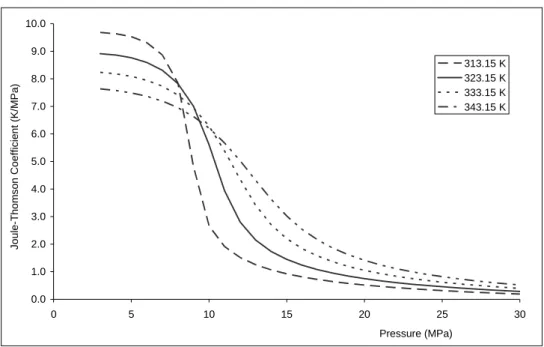
where T is the temperature, P is the pressure, and H is a partial derivative at constant enthalpy. Figure 1 shows that Joule-Thomson coefficients are greater at low pressure than at pressures higher than 7 MPa, i.e. about 0.5 K/MPa at 40 °C and 20 MPa and about 20 times higher at the same temperature and 5 MPa.
Therefore the Joule-Thomson effect will be greatest in cases of CO2 storage in depleted gas fields with low pressure (e.g., Oldenburg 2007). For CO2 storage in saline aquifers at depths greater than 700 m (pressure higher than 7 MPa), a weak Joule-Thomson effect is expected (Bielinski et al. 2008). Nevertheless, even if this thermal effect is limited in deep aquifers and hydrodynamic and transport properties are weakly influenced by cooling, the amplitude of the Joule-Thomson coefficient is non-negligible and may combine with other thermal processes (described above) to induce a significant cumulative effect.
0.0 1.0 2.0 3.0 4.0 5.0 6.0 7.0 8.0 9.0 10.0
0 5 10 15 20 25 30
Pressure (MPa)
Joule-Thomson Coefficient (K/MPa)
313.15 K 323.15 K 333.15 K 343.15 K
Figure 1: Joule-Thomson coefficient for CO2 as a function of pressure and temperature (data from NIST Webbook).
2.5 Injection temperature
Downhole injection temperature will control many fundamental processes (e.g., thermo-chemical, thermo-mechanical). This injection temperature is dependent on the PVTX properties (pressure, volume, temperature and composition) of the injected gas stream. It also depends on wellhead conditions (which are subject to operational, economic, legal, engineering, and safety constraints), well
completion, and many other parameters such as pressure losses and heat exchange along the wellbore. Phase changes can be expected in the well for specific cases due to these complex thermodynamic processes. The determination of downhole temperature has not yet received much attention and few bibliographic data exist.
Bielinski et al. (2008) suggested a downhole CO2 temperature ranging from 40 to 60 °C for an injection well targeting a host reservoir about 700 m deep with an initial temperature between 33 and 36 °C. Some recent papers present also attempts to model CO2 flow in the injection wellbore (Pruess 2004; Lu and Connell 2008; Pan et al. 2008; Paterson et al. 2008).
3 Numerical tool and modelling approach
3.1 Numerical tool
The TOUGHREACT simulator (Xu and Pruess 2001) was used for all the simulations in this study. This code couples thermal, hydrologic and chemical (THC) processes and is applicable to one-, two-, or three-dimensional geologic systems with physical and chemical heterogeneity. ECO2n (Pruess 2005), a fluid property module for TOUGH2 V2 (Pruess et al. 1999) was developed specifically to model isothermal or non-isothermal multiphase flow in water/brine/CO2
systems. Actually, apart the heat transfer through confining beds, all the other processes presented in section 2 derives from the description of thermodynamics which is accomplished by ECO2n for H2O-CO2-NaCl mixtures.
TOUGHREACT simulates the chemical reactivity of the system based on a thermodynamic database, which is an extension of the EQ3/6 database (Wolery 1992) for the 0–300 °C range, 1 bar below 100 °C, and water saturation pressure above 100 °C.
The current TOUGHREACT version uses an extended Debye-Hückel model (Helgeson et al. 1981) to determine activity coefficients of dissolved species:
( ) Log(1 0.0180153m*)
[
b b 0.19(z 1)]
II B a 1
I z
Log A i NaCl Na,Cl i
2 / o 1
2 2 i
i + + − ω + − −
+
−
=
γ + −
γ
γ (2)
where i refers to each ion, γ is the activity coefficient of the ion, z is the ion electric charge, m* is the total molality of all species in solution, I is taken as the true ionic strength of the solution, ω is the Born coefficient, bNa+,Cl-, bNaCl, are Debye-Hückel parameters and å is calculated from ion radii.
Aγ and Bγ, temperature and pressure dependent parameters, were calculated according to Lassin et al. (2005). The new values for Aγ and Bγ are 0.5568 kg1/2 mol-1/2 and 0.3367 1010 kg1/2 mol-1/2 m-1 at 200 bars and 75 °C, respectively, compared to 0.5095 kg1/2 mol-1/2 and 0.3284 1010 kg1/2 mol-1/2 m-1 at 1 bar pressure and 25 °C.
André et al. (2007) did calculations with TOUGHREACT and an in-house code, SCALE2000 (Azaroual et al. 2004), a geochemical simulator designed for highly saline solutions. There are discrepancies between the two codes and conclusions highlight the advantage of using the Pitzer formalism rather the Debye-Hückel for ionic strength higher than 0.5 - 0.7. Nevertheless, TOUGHREACT enables a first qualitative approach to the main geochemical processes and general evolutionary trends of the system.
Mineral dissolution and precipitation reactions occur under kinetic conditions.
The general form of the rate law proposed by Lasaga (1984) and Steefel and Lasaga (1994) is applied for mineral dissolution and precipitation:
θ η
Ω
−
±
= n n n
n k A 1
r (3)
A positive value for rn (mol s-1) corresponds to dissolution of the mineral n (negative for precipitation), kn is the rate constant (mol m-2 s-1) depending on the temperature, An is the specific reactive surface area (m2 kgw-1), and Ωn is the saturation ratio of the mineral n (Ωn = Q/K). The empirical parameters θ and η are determined from experiments, otherwise they are usually taken as 1.
The dependence of the rate constant k with temperature is calculated by means of the Arrhenius equation:
⎥⎦
⎢ ⎤
⎣
⎡ ⎟
⎠
⎜ ⎞
⎝⎛ −
= −
15 . 298
1 T 1 R exp E k
k 25 a (4)
where Ea (J mol-1) is the activation energy, k25 (mol m-2 s-1) the rate constant at 25°C, R (J K-1 mol-1) is the universal gas constant and T (K) the absolute temperature.
The dissolution and precipitation of alumino-silicates and salts can be controlled by the H+ concentration (acid mechanism) and the OH- concentration (alkaline mechanism) in addition to the neutral mechanism corresponding to Equation 4. In this case, rn is calculated using the following extended equation:
θ η
Ω
−
⎥⎥
⎥⎥
⎥⎥
⎥⎥
⎥
⎦
⎤
⎢⎢
⎢⎢
⎢⎢
⎢⎢
⎢
⎣
⎡
⎥⎥
⎦
⎤
⎢⎢
⎣
⎡ ⎟
⎠
⎜ ⎞
⎝⎛ − + −
⎥⎥
⎦
⎤
⎢⎢
⎣
⎡ ⎟
⎠
⎜ ⎞
⎝⎛ − + −
⎥⎥
⎦
⎤
⎢⎢
⎣
⎡ ⎟
⎠
⎜ ⎞
⎝⎛ −
−
= n n
nOH H OHa
OH25
nH H Ha
H25 nua nu25
n A 1
15 a . 298
1 T 1 R exp E k
15 a . 298
1 T 1 R exp E k
15 . 298
1 T 1 R exp E k
r (5)
where superscripts or subscripts nu, H and OH indicate neutral, acid and alkaline mechanisms, respectively, and a is the activity of the corresponding species.
For carbonate minerals, dissolution/precipitation mechanisms are catalyzed by bicarbonate ions (HCO3-) and reaction rates depend on the activity of aqueous CO2 (carbonates mechanism). In this case, rn is calculated using the following equation:
θ η
Ω
−
⎥⎥
⎥⎥
⎥⎥
⎥⎥
⎥
⎦
⎤
⎢⎢
⎢⎢
⎢⎢
⎢⎢
⎢
⎣
⎡
⎥⎥
⎦
⎤
⎢⎢
⎣
⎡ ⎟
⎠
⎜ ⎞
⎝⎛ − + −
⎥⎥
⎦
⎤
⎢⎢
⎣
⎡ ⎟
⎠
⎜ ⎞
⎝⎛ − + −
⎥⎥
⎦
⎤
⎢⎢
⎣
⎡ ⎟
⎠
⎜ ⎞
⎝⎛ −
−
= n n
2 nCO
aq , CO2 2
COa CO2
25
nH H H
a H25
nu nu a
25
n A 1
15 a . 298
1 T 1 R exp E k
15 a . 298
1 T 1 R exp E k
15 . 298
1 T 1 R exp E k
r (6)
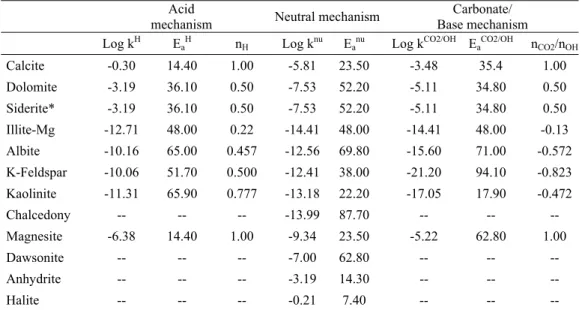
The parameters in the kinetic rate equation are shown in Table 1. Acid-catalyzed, base-catalyzed and neutral kinetic mechanisms are used in this simulation.
Table 1: Kinetic parameters for mineral dissolution and precipitation (Palandri & Kharaka, 2004) Acid
mechanism Neutral mechanism Carbonate/
Base mechanism Log kH EaH nH Log knu Eanu Log kCO2/OH EaCO2/OH nCO2/nOH
Calcite -0.30 14.40 1.00 -5.81 23.50 -3.48 35.4 1.00 Dolomite -3.19 36.10 0.50 -7.53 52.20 -5.11 34.80 0.50 Siderite* -3.19 36.10 0.50 -7.53 52.20 -5.11 34.80 0.50 Illite-Mg -12.71 48.00 0.22 -14.41 48.00 -14.41 48.00 -0.13 Albite -10.16 65.00 0.457 -12.56 69.80 -15.60 71.00 -0.572 K-Feldspar -10.06 51.70 0.500 -12.41 38.00 -21.20 94.10 -0.823 Kaolinite -11.31 65.90 0.777 -13.18 22.20 -17.05 17.90 -0.472 Chalcedony -- -- -- -13.99 87.70 -- -- -- Magnesite -6.38 14.40 1.00 -9.34 23.50 -5.22 62.80 1.00 Dawsonite -- -- -- -7.00 62.80 -- -- -- Anhydrite -- -- -- -3.19 14.30 -- -- --
Halite -- -- -- -0.21 7.40 -- -- --
*Kinetic data for siderite are assumed to be equivalent of those of dolomite (Gunter et al. 2000)
Following the mineral dissolution and precipitation, the reservoir porosity and permeability are calculated at each time step. Porosity changes in the matrix are directly related to the volume changes resulting from mineral precipitation and dissolution. Matrix permeability changes are calculated from porosity changes using the Carman-Kozeny relationship (Bear 1972). The poor knowledge of the structural characteristics of the investigated reservoir rock prevented the use of more complex porosity/permeability relationships depending on factors, such as pore size distribution, pore shapes, and connectivity. Changes in porosity and permeability also have an impact on capillary pressure which is upscaled using the Leverett scaling relation (Slider 1976). These calculations are done in the
chemical part of TOUGHREACT and the feedback effect of changes in porosity, permeability, and capillary pressure is considered on fluid flow calculations in the hydrodynamic part of the code.
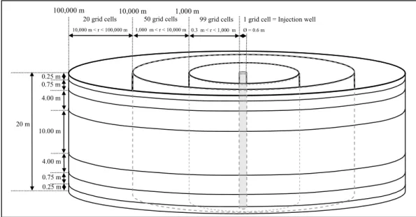
3.2 Geometrical model
A 2D radial model is proposed as a conceptual framework for determining the transient evolution of the geochemical reactivity induced by the injection of CO2. The 20-m-thick reservoir is centred on a vertical injection well (Figure 2). The maximum radial extent is 100 km. The system under consideration is represented by 1190 grid blocks comprising the model mesh. The radius of the injection cell is 0.3 m. Along the radius axis, 99 grid cells are considered between 0.3 and 1000 m, 50 grid cells between 1000 m and 10 km, and 20 grid cells between 10 and 100 km. In each interval, the width of the radial elements follows a logarithmic scale.
The objective of such refinement near the injection well is to capture more precisely both the details of geochemical processes and the migration of the desiccation front in the near-well region. The vertical discretization is achieved by a division of the reservoir into seven layers. The seven reservoir layers are, from bottom to top, 0.25, 0.75, 4, 10, 4, 0.75 and 0.25 m thick.
99 grid cells 0.3 m < r < 1,000 m 50 grid cells
1,000 m < r < 10,000 m
1 grid cell = Injection well Ø = 0.6 m
1,000 m 10,000 m
100,000 m
10,000 m < r < 100,000 m
20 m 0.25 m 0.75 m 4.00 m
4.00 m 0.75 m 0.25 m 10.00 m
20 grid cells
Figure 2: Geometrical 2D radial model for supercritical CO2 injection in a carbonate reservoir. The diameter of the injection well is 0.6 m whereas the first element adjacent to the wellbore presents a width of 0.32 m.
The bedrock and caprock are assumed to be impervious, whereas thermal conduction from the bedrock and caprock to the reservoir is taken into account.
In TOUGH2, the method of Vinsome and Westerveld (1980) is used to integrate heat exchanges between reservoir fluids and the confining beds. This method is based on a semi-analytical approach that prevents meshing outside of the fluid flow domain. The vertical layers close to the bedrock and caprock are thinner in agreement with the numerical constraints of vertical heat exchanges (i.e. thermal gradient, heat conductivity, time step, etc.).
No regional flow is considered and a hydrostatic status is initially assumed for the pressure within the reservoir and maintained constant at the lateral boundary. The initial temperature and pressure of the targeted reservoir are 75 °C and 18 MPa, respectively.
The physical properties of the reservoir are those of the Dogger aquifer in the Paris Basin. This regional reservoir, with a mean depth of 1600-1700 m, has a porosity of 0.15. Reservoir permeability is anisotropic, with a horizontal
permeability of 10-13 m² (100 mD) and a vertical permeability of 10-14 m² (10 mD) (KV/KH = 0.1). Mainly composed of carbonates, its rock grain density approaches 2750 kg m-3. The formation heat conductivity and the rock grain specific heat are 2.51 W/m °C and 900 J/kg °C, respectively (Rojas et al. 1989).
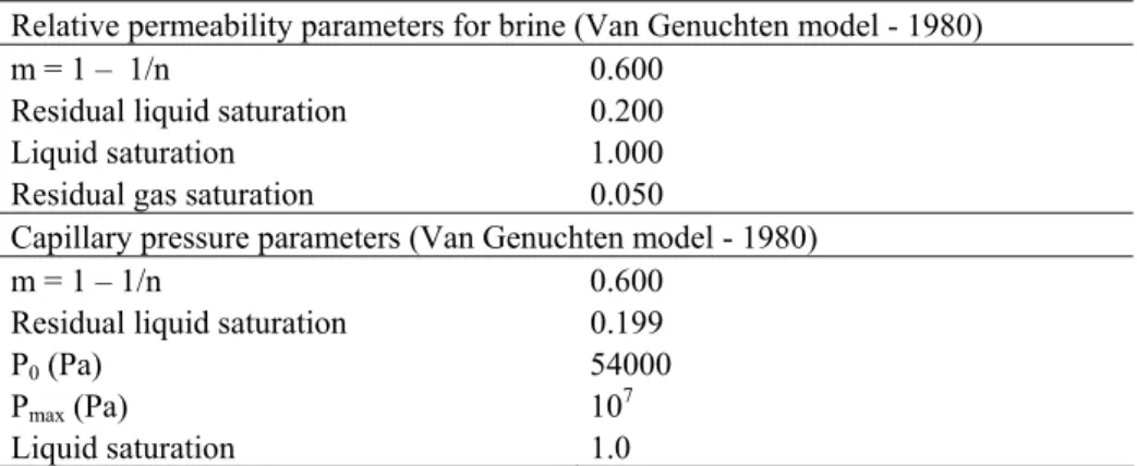
The experimental capillary pressure and the liquid relative permeability were fitted using the Van Genuchten model, whereas gas relative permeability was fitted with a fourth-degree polynomial function (André et al. 2007). The parameters used in the simulations for liquid relative permeability and capillary pressure models are summarized in Table 2.
Table 2: Van Genuchten parameters used for fitting the characteristic curves for brine (i.e., relative permeability and capillary pressure), whereas a polynomial correlation was used for the relative permeability of the gas phase (see André et al. 2007 for greater detail).
Relative permeability parameters for brine (Van Genuchten model - 1980)
m = 1 – 1/n 0.600
Residual liquid saturation 0.200
Liquid saturation 1.000
Residual gas saturation 0.050
Capillary pressure parameters (Van Genuchten model - 1980)
m = 1 – 1/n 0.600
Residual liquid saturation 0.199
P0 (Pa) 54000
Pmax (Pa) 107
Liquid saturation 1.0
During the brine evaporation process driven by dry CO2 injection, the capillary pressure is limited to a maximum value of 10 MPa. This value is quite large but it is not unreasonable compared to values proposed by many authors who predict values up to 100 MPa during the desiccation process of a porous medium (Rossi and Nimmo 1994; Pettenatti et al. 2008 and references cited therein).
3.3 Mineralogical assemblage
The Dogger reservoir consists mainly of carbonates (85% by volume calcite, disordered dolomite and siderite) with some alumino-silicates (albite and K- Feldspar) and illite (Rojas et al. 1989). Minerals that can precipitate as secondary phases during CO2 injection are kaolinite, chalcedony, magnesite, dawsonite, anhydrite and halite (Table 3).
Table 3: Dogger aquifer mineralogy and list of minerals not initially present in the reservoir but able to precipitate
Mineral composition Volume fraction
Calcite 0.70 Dolomite 0.10 Siderite 0.05 Illite 0.05 Albite 0.05 Primary minerals
K-feldspar 0.05 Kaolinite 0.00 Chalcedony 0.00 Magnesite 0.00 Dawsonite 0.00 Anhydrite 0.00 Secondary minerals
(potentially precipitating minerals)
Halite 0.00
3.4 Water chemistry
While the Dogger reservoir contains water with salinity values ranging from moderate (3 g kg-1 of water) to high (35 g kg-1 of waterin the deepest part of the aquifer), in this study, only a moderately saline brine (5 g kg-1 of water) is assumed (Table 4) (Michard and Bastide 1988). This water is initially at
thermodynamic equilibrium with all the minerals initially present in the reservoir.
The partial pressure of carbon dioxide (pCO2 ) governs the equilibrium of the solution with calcite and the pH of the water results from this equilibrium with carbonate rocks (calcite and disordered dolomite) (Michard and Bastide 1988).
Silicon concentration is correlated to reservoir temperature and is in agreement with chalcedony solubility (Azaroual et al. 1997).
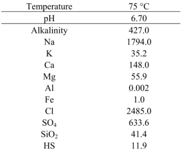
Table 4: Chemical composition of Dogger aquifer water in the low salinity part of the reservoir (concentrations in ppm)
Temperature 75 °C
pH 6.70 Alkalinity 427.0
Na 1794.0 K 35.2 Ca 148.0 Mg 55.9 Al 0.002 Fe 1.0 Cl 2485.0
SO4 633.6
SiO2 41.4
HS 11.9
4 Numerical simulations
The results of two injection scenarios are presented here. The numerical simulations were done by coupling thermal, hydraulic and chemical processes (THC simulations). The first scenario uses a low injection flow rate (1 kg s-1) and the second, a high injection flow rate (20 kg s-1). For Scenario 1, two injection temperatures are used: 75 °C and 40 °C. The higher temperature (i.e. the reservoir temperature) is used to highlight the role of internal thermal effects (role of
petrophysical properties and thermodynamic constraints). The lower temperature was selected in order to have a maximum difference relative to the reservoir temperature (with an anthropic origin) but also to maintain CO2 in the supercritical state.
The specified downhole temperatures are constant for the two scenarios during the entire injection period and the injected CO2 is dry (absolutely no water). The CO2
is injected into the thickest layer of the reservoir, i.e. the 10-m layer at mid-depth in order to increase the pressure gradient close to the injection well and thus, amplify thermal processes as the Joule-Thomson effect.
In this study, the injection period is quite short (about 300 days) because only the near-well region is explored. The reactivity close to the injection well is
emphasized because it will have a direct impact on well injectivity and the integrity of the well completion.
4.1 Scenario 1: coupled simulations (THC) at low flow rate (1 kg s-1)
Supercritical CO2 is injected at a very low flow rate (1 kg s-1) enabling us to define and quantify the major physical, thermal, and geochemical processes occurring in the near-well region and within the reservoir at different spatial and time scales. The injection temperatures are 75 °C (Scenario 1A) and 40 °C
(Scenario 1B). The objective of Scenario 1A is to verify the conclusions in André et al. (2007) and to determine whether the geometrical model (2D radial vs. 1D radial) has an impact on the results. Scenario 1B is used to determine the role of temperature on chemical reactivity.
4.1.1 Within the entire impacted area (large scale)
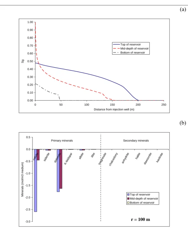
The injection of CO2 causes a small increase in pressure. The maximum build up occurs near the well (with an increase of about 0.5 MPa) but the pressure impact has spread 5,000 m around the injection well after 300 days. A second key point concerns the extension of the gas bubble and the position of the two-phase front within the reservoir. As CO2 solubility in water at this pressure and temperature is about 1 mol kg-1w, all the injected CO2 cannot be dissolved in the formation water and a two-phase system (supercritical CO2 – saline water) develops within the reservoir. The injected CO2 pushes the formation water away from the injection well by a piston-like effect. After 300 days, the gas bubble extends about 200 m around the injection well at the top of the reservoir and 50 m at the bottom (Fig. 3a). The spreading is not uniform within the reservoir due to relative
permeability and viscosity effects (phase mobility) against gravity forces. This simulation also shows that with such an injection period and low flow rate (1 kg s-
1), no desiccation occurs close to the injection well.
The chemical composition of the groundwater in the reservoir is impacted by the injected CO2. Carbon dioxide dissolution increases the acidity of the medium, enabling mineral dissolution (mainly of carbonates). The groundwater pH is buffered to about 4.8 because of the equilibrium between the water and carbonate minerals. As the radius of the CO2 bubble increases, the flowing brine
composition in the area between the two-phase displacement front and the dry-out front is governed by gas-fluid-rock exchanges. This thermodynamic equilibrium state between these phases does not permit to dissolve more and more carbonates during the brine flow preventing any massive spatially localised dissolution of native reservoir minerals. However, due to the shape of the gas front,
mineralogical reactivity is greater at the top of the reservoir (Fig. 3b). Calcite is the most reactive mineral, with dissolved quantities 5-times greater near the interface with the caprock than at mid-depth in the reservoir. Dolomite does not present the same behaviour, with a more regular dissolution in the upper part of the reservoir. Some weak dissolutions of siderite, albite and K-Feldspar are also observed in the upper part of the reservoir. The spatial variations of chemical reactivity depend only on CO2 concentration and pH (no thermal effect, Fig. 4).
As CO2 moves upward into the aquifer, the acidity increases at the top of the reservoir and mineral dissolution occurs, in particular near the interface with the caprock. Near the interface with the basement, the reactivity is negligible because the CO2 does not reach this region.
Far from the injection well (100 to 250 m), the temperature effects are insignificant and only the heat-of-dissolution of CO is observable (Fig. 4).
However, this temperature increase alone cannot explain the differences in chemical reactivity.
(a)
0.00 0.10 0.20 0.30 0.40 0.50 0.60 0.70 0.80 0.90 1.00
0 50 100 150 200 250
Distance from injection well (m)
Sg
Top of reservoir Mid-depth of reservoir Bottom of reservoir
(b)
-3.0 -2.5 -2.0 -1.5 -1.0 -0.5 0.0 0.5
calcite siderite
dolomite K-feldspar
albite illite
magnesite chalcedony
anhydrite halite
dawsonite kaolinite
Minerals (mol/m3 medium)
Top of reservoir Mid-depth of reservoir Bottom of reservoir
Primary minerals Secondary minerals
r = 100 m
Figure 3: Results obtained with Scenario 1A: (a) Spatial evolution of gas saturation within the reservoir after a 300-day period of supercritical CO2 injection at 1 kg s-1 and 75 °C; (b) Quantity of dissolved minerals (mostly carbonates) 100 m from the injection well.
4.1.2 Within 10 metres of the injector (near-well region)
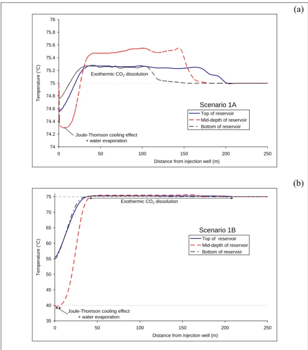
Thermal effects are greater near the injection well (0 to 50 m, Fig. 4). Many thermal processes are involved, e.g. the Joule-Thomson cooling effect and the
enthalpy of water evaporation close to the well. Due to the weak pressure gradient at this injection rate, the Joule-Thomson cooling effect is, however, small, with variations of about 1 °C.
(a)
74 74.2 74.4 74.6 74.8 75 75.2 75.4 75.6 75.8 76
0 50 100 150 200 250
Distance from injection well (m)
Temperature (°C)
Top of reservoir Mid-depth of reservoir Bottom of reservoir Joule-Thomson cooling effect
+ water evaporation Exothermic CO2 dissolution
Scenario 1A
(b)
35 40 45 50 55 60 65 70 75
0 50 100 150 200 250
Distance from injection well (m)
Temperature (°C) Top of reservoir
Mid-depth of reservoir Bottom of reservoir
Joule-Thomson cooling effect + water evaporation
Exothermic CO2 dissolution
Scenario 1B
Figure 4: Spatial evolution of temperature within the reservoir after a 300-day period of supercritical CO2 injection at 1 kg s-1: (a) at 75 °C; (b) at 40 °C. (Note: The scale is different in figures a and b). Grey dashed lines represent the initial reservoir temperature (75 °C).
For Scenario 1A, the temperature gradients are very low (Fig. 4a). The
consequence is a weak influence of temperature on mineralogical reactivity. This is confirmed at 10 m from the injector, a zone where the CO2 concentration is
quite constant on a vertical profile (Fig. 3a). The dissolution of carbonates (dolomite, calcite and siderite) and other primary minerals (albite, K-Feldspar) is homogeneous (Fig. 5a).
(a)
-3.0 -2.0 -1.0 0.0 1.0 2.0 3.0 4.0 5.0
calcite siderite
dolomite K-feldspar
albite illite magnesite
chalcedony anhydrite
halite dawsonite
kaolinite
Minerals (mol/m3 medium) Top of reservoir
Mid-depth of reservoir Bottom of reservoir
Primary minerals Secondary minerals
r = 10 m
(b)
-3.0 -2.0 -1.0 0.0 1.0 2.0 3.0 4.0 5.0
calcite siderite
dolomite K-feldspar
albite illite
magnesite chalcedony
anhydrite halite
dawsonite kaolinite
Minerals (mol/m3 medium)
Top of reservoir Mid-depth of reservoir Bottom of reservoir
Primary minerals Secondary minerals
r = 1 m
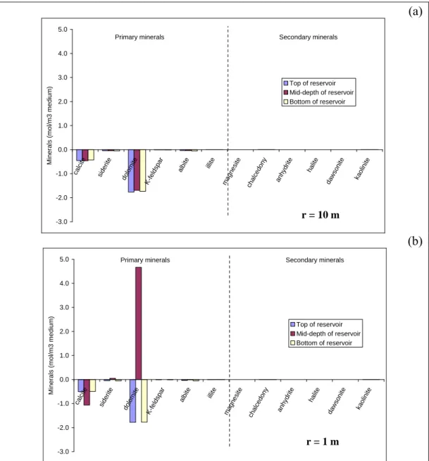
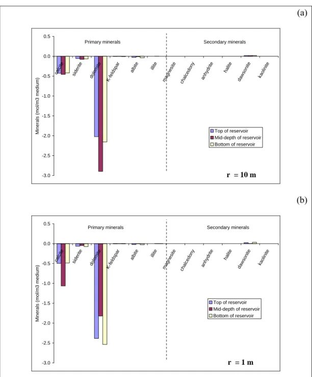
Figure 5: Results obtained with Scenario 1A - Variations in mineral concentrations around the injection well after a 300-day period of supercritical CO2 injection (flow rate = 1 kg s-1 and T = 75
°C): (a) 10 m; (b) 1 m. Negative values correspond to dissolution and positive values to precipitation.
Closer to the injector, the behaviour of different minerals is highly variable (Fig.
5b). As dry CO2 is injected at mid-depth in the reservoir, water evaporation occurs preferentially. Residual water, trapped in micropores, evaporates and
minerals can precipitate. Dolomite and siderite precipitate, whereas calcite continues to dissolve (Fig. 5b). Because the CO2 injection flow rate is low, the desiccation process does not appear to be advanced enough to enable the precipitation of salts. Only primary minerals are affected by this process.
For Scenario 1B, Figure 4b clearly shows that major temperature gradients are observed in the first 10 metres from the injection well, mainly due to the injection temperature (Tinj = 40 °C). The temperature is not uniform within the reservoir and differences of about 20 °C are expected between reservoir mid-depth and reservoir edges. Consequently, highly variable mineralogical reactivity is
expected in this zone (Fig. 6). Ten meters from the injector, dolomite dissolution is about 50 % greater at reservoir mid-depth than at the reservoir edges (Fig. 6a).
The difference in chemical reactivity is essentially caused by temperature effects:
low temperatures increase both CO2 dissolution and carbonate solubility
(Plummer and Busenberg 1982). One meter from the injection well, there is more calcite dissolution at reservoir mid-depth than close to the interfaces with the caprock and basement, whereas there is 25 % less dissolution of dolomite and siderite at reservoir mid-depth than on the edges (Fig. 6b). An explanation for this can be seen in Figure 7. First, there is more dolomite and siderite dissolution in Scenario 1B than in Scenario 1A due to a low injection temperature. Second, because of desiccation, the dolomite and siderite precipitation period follows the dissolution period at mid-depth in the reservoir.
(a)
-3.0 -2.5 -2.0 -1.5 -1.0 -0.5 0.0 0.5
calcite siderite
dolomite K-feldspar
albite illite
magnesite chalcedony
anhydrite halite
dawsonite kaolinite
Minerals (mol/m3 medium)
Top of reservoir Mid-depth of reservoir Bottom of reservoir
Primary minerals Secondary minerals
r = 10 m
(b)
-3.0 -2.5 -2.0 -1.5 -1.0 -0.5 0.0 0.5
calcite siderite
dolomite K-feldspar
albite illite
magnesite chalcedony
anhydrite halite
dawsonite kaolinite
Minerals (mol/m3 medium)
Top of reservoir Mid-depth of reservoir Bottom of reservoir
Primary minerals Secondary minerals
r = 1 m
Figure 6: Results obtained from Scenario 1B - Variation in mineral concentrations around the injection well after a 300-day period of supercritical CO2 injection (flow rate = 1 kg s-1 and T = 40
°C): (a) 10 m; (b) 1 m. Negative values correspond to dissolution and positive values to precipitation.
The start of this phase and its magnitude differ in Scenarios 1A and 1B: dolomite and siderite precipitation begins 100 days later and with a lower magnitude in Scenario 1B. The geochemical process seems to be influenced by temperature with larger dolomite and siderite deposits at 75 °C (Fig. 5b) than at 40 °C (Fig.
6b). Precipitation of dawsonite also seems to be temperature-dependent. No deposits are observed at 75 °C whereas some precipitation is observed at 40 °C.
Traces of dawsonite are observed mainly on the edges of the reservoir, 1 and 10 m from the injection well (Fig. 6).
(a)
-3.0 -2.0 -1.0 0.0 1.0 2.0 3.0 4.0 5.0
0 50 100 150 200 250 300
Time (days)
Dolomite (mol/m3 medium)
Case 1A
Case 1B
r = 1 m
(b)
-0.10 -0.08 -0.06 -0.04 -0.02 0.00 0.02 0.04 0.06 0.08 0.10
0 50 100 150 200 250 300
Time (days)
Siderite (mol/m3 medium)
Case 1A
Case 1B
r = 1 m
Figure 7: Variation in dolomite (a) and siderite (b) concentrations 1 m from the injection well at mid-depth in the reservoir for Scenarios 1A and 1B.
The impact of temperature on dolomite reactivity can be clearly seen when the dolomite concentration around the injection well is plotted for Scenarios 1A and
1B (Fig. 8). Dolomite dissolution is greater in Scenario 1B in the reservoir zone where the temperature is lower than 60 °C (Fig. 4b). A dissolution ratio of 2 is observed between the low temperature zone (0 to 30 m) and the high temperature zone (beyond 30 m).
-3.00 -2.00 -1.00 0.00 1.00 2.00 3.00 4.00 5.00
0 20 40 60 80 100 120 140 160 180 200
Distance from injection well (m)
Dolomite (mol/m3 medium)
Case 1B Case 1A
Thermal front
Hydraulic fronts dependant on injection temperature
Figure 8: Relative variations of dolomite concentration after a 300-day period of supercritical CO2
injection in the reservoir mid-depth for the Scenarios 1A and 1B.
The results using Scenario 1A are in good agreement with previous results obtained on a 1D radial model (André et al. 2007). 1D and 2D calculations confirm that, in a first step, the injection of CO2 into a carbonate reservoir causes the dissolution of carbonates (calcite, dolomite, siderite). Other primary minerals such as albite and K-Feldspar also dissolve due to acidification, but to a lesser extent. Furthermore, the 1D and 2D approaches both show that the near-well region (less than 5 m from injector) is affected by mineral precipitation. Dolomite seems to be the most reactive mineral and it precipitates first. The 1D simulation was done with a long-term injection period (10 years) and salt precipitation (anhydrite) was observed. The simulation period in Scenario 1A (300 days) is too short to observe this type of phenomenon. Nevertheless, this 2D approach goes
further than the 1D approach and enables us to predict the spatial reactivity of the system. While the 1D calculation gave simply the radius of mineral precipitation, the 2D model provides information concerning the vertical position of the
deposits and the architectural structure of active geochemical reactions.
4.2 Scenario 2: coupled simulation (THC) at high flow rate (20 kg s-1) and injection temperature of 40 °C
This numerical simulation uses a scenario in which supercritical CO2 is injected at an industrial flow rate (20 kg s-1) and a temperature of 40 °C, lower than the initial reservoir temperature. The aim is to determine the impact of reservoir cooling, induced by a massive injection of CO2, on chemical reactivity.
4.2.1 Within the entire impacted area (large scale)
Whereas reservoir pressure was not significantly affected by CO2 injection in Scenario 1, supercritical CO2 injection at a higher flow rate (x 20) causes a large increase in pressure throughout the reservoir. In the first 20 km around the injection well, the pressure grows, with a maximum increase from 18 MPa to up to 23.5 MPa close to the injection well (Fig. 9a). As injected gas moves into the mid-depth of the reservoir, the maximum build-up of pressure is significant in the centre of the aquifer. Pressure near the interfaces is quite similar with higher values at the bottom of the reservoir due to gravity. Beyond 40 m, the pressure gradient between the top and the bottom of the reservoir does not exceed 0.2 MPa (Fig. 9a).
Similar to what occurs in Scenario 1, the massive CO2 injection leads to the formation of a two-phase system (supercritical CO2 and brine). Depending on temperature and pressure conditions, part of the injected CO2 dissolves in the groundwater whereas the remaining CO2 stays in its own supercritical state.
Figure 9b shows the evolution of gas (supercritical) saturation within the
reservoir. After 300 days of injection, desiccation occurs in the grid cells located at mid-depth in the reservoir within a radius of about 20 m. Although the
injection flow rate is high, the CO2 distribution in the reservoir is driven by an upward movement of supercritical CO2 close to the top interface (Fig. 9b).
Far from the injection well (100 to 300 m), the chemical reactivity at a given vertical profile is constant. Figure 10 shows that carbonates, in particular, are affected by CO2 injection. While calcite and dolomite are the most dissolved minerals, siderite, albite and K-Feldspar are also impacted by acidification of the medium. The similarity of figures 10 and 5a is very interesting. It shows that the injection flow rate does not have an impact on elementary and fundamental chemical processes (carbonate and mineral dissolution) but only on the location within the reservoir where these processes occur. With the increase in the injection flow rate, the chemical processes occur farther from the injector.
(a)
17.5 18.5 19.5 20.5 21.5 22.5 23.5 24.5
0 5000 10000 15000 20000
Distance from injection well (m)
Pressure (Mpa)
Top of reservoir Mid-depth of reservoir Bottom of reservoir
Initial reservoir pressure
21.0 21.5 22.0 22.5 23.0 23.5
0 20 40 60 80 100 120 140
Distance from injection well (m)
Pressure (Mpa)
(b)
0.0 0.2 0.4 0.6 0.8 1.0
0 250 500 750
Distance from injection well (m)
Sg
Top of reservoir Mid-depth of reservoir Bottom of reservoir
Figure 9: Results obtained with Scenario 2 after a 300-day period of supercritical CO2 injection at 20 kg s-1 and 40 °C: (a) Spatial evolution of pressure within the reservoir (with enlargement of 0 to 150 m); (b) Spatial evolution of gas saturation within the reservoir.
-3.5 -3.0 -2.5 -2.0 -1.5 -1.0 -0.5 0.0 0.5
calcite siderite
dolomite K-feldspar
albite illite magnesite
chalcedony anhydrite
halite dawsonite
kaolinite
Mineral (mol/m3 medium)
Top of reservoir Mid-depth of reservoir Bottom of reservoir
Primary minerals Secondary minerals
r = 100 m
Figure 10: Results obtained with Scenario 2 - Variation in mineral concentrations 100 m from the injection well after a 300-day period of supercritical CO2 injection (flow rate = 20 kg s-1 and T = 40 °C).
4.2.2 Within 100 metres of the injector (near-well region)
The injection of cold supercritical CO2 (40 °C) causes a decrease in temperature in the near-well region. Different processes can be identified (Fig. 11):
- In the first 20 metres, where desiccation is total, the Joule-Thomson effect is expressed. It is about 1 °C, correlated to the pressure gradient presented in Figure 9a.
- Between 20 and 50 metres, a greater decrease of temperature is observed (enlargement in Figure 11). Some of this temperature gradient is due to the Joule-Thomson effect (in the same order of magnitude as what was observed between 0 and 20 m), whereas another part is due to water evaporation. In this zone, the temperature gradient between the mid-depth and the edges of the reservoir is greatest and reaches 10 to 15 °C
depending on the location in the reservoir and the period of CO2 injection.
- Between 50 and 100 metres, the temperature increases gradually. The thermal front moves into the reservoir as a function of the imposed flow rate.