Jean Ponce Professeur, Directeur DI, Directeur de thèse ENS Ulm Pedro Felzenszwalb Professeur, Brown University Reporter. Ils m’ont tous profondément influencé et m’ont aidé à améliorer ma façon de faire des recherches.
Background
However, vision is complex: macaques use 60 percent of their brain for visual perception [Vanduffel et al., 2002], and humans use even more in terms of absolute size. Therefore, humans can see without even noticing how complex and difficult this task is, and unlike many other areas of computer science, computer vision still lags far behind human-level performance.
Motivation and aim of study
- Building a category-level object detector
- Aligning to build a similarity measure
- A direct approach to the misalignment problem
- Aligning rigid objects
- Aligning deformable objects
Using only the local view, it will simply match each part of the first image with the most similar part in the second image. Rather, here, each part of the prototype can potentially match anywhere in the test image.
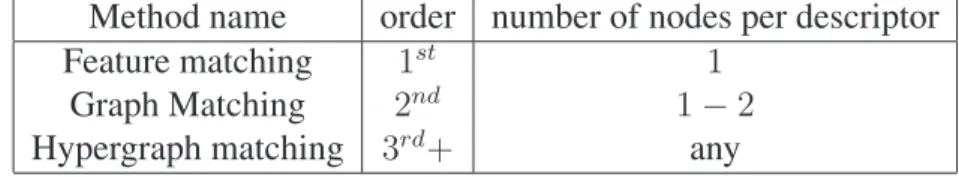
Graph matching
A unary part, which encourages nodes of the first graph to be linked to similar nodes, e.g. A binary part, which encourages node pairs of the first graph to be linked to node pairs of the second graph, with a similar geometric relationship (see Figure 1.10 and caption).
Objective and contributions of the thesis
Motivation and goals
Applications of graph matching for object detection and recognition are presented in the following chapters. The simplest approach to this problem is to define a similarity measure between two features (eg, the Euclidean distance between SIFT descriptors of small image patches [Lowe, 2004a]), and match each feature to the first image .
Problem statement
Organization and Contributions
Previous work
Historical review of literature
At one end of the spectrum, geometric matching techniques such as RANSAC [Fischler and Bolles, 1981], interpretation trees [Grimson and Lozano-Pérez, 1987], or alignment [Huttenlocher and Ullman, 1987b] can be used to efficiently explore. consistent correspondence hypotheses when the mapping between image features is assumed to have some parametric form (e.g. a planar affine transformation), or to obey certain parametric constraints (e.g. epipolar constraints). Modern methods for image matching now tend to mix both geometric and appearance cues to guide the search for similarities (see for example [Lazebnik et al., 2006a; Lowe, 2004a]).
Spectral matching
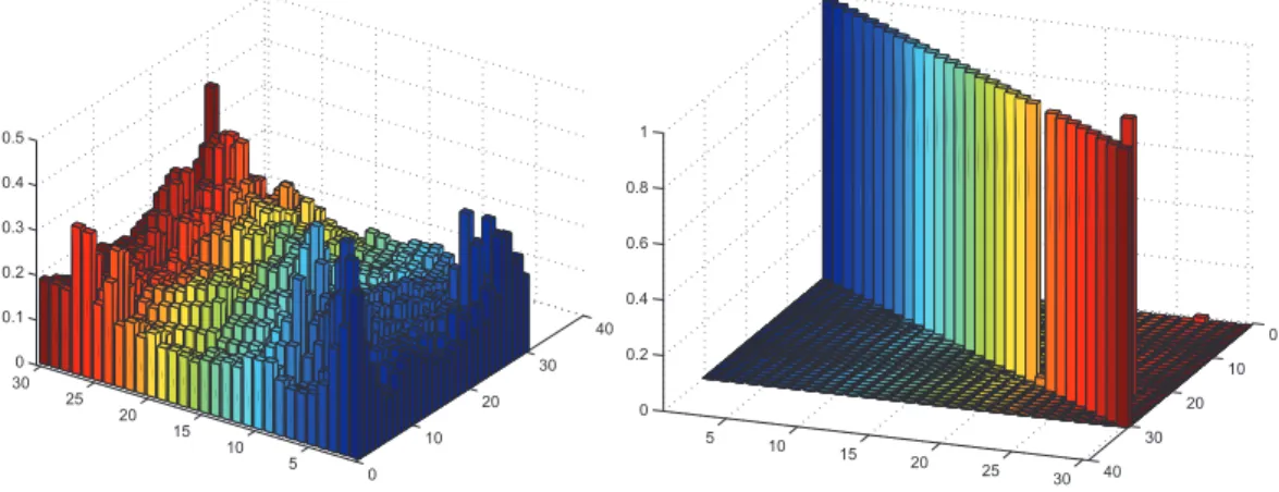
X˜TH˜X, where˜ X˜ denotes the vector in RN1N2 obtained by concatenating the columns of X and likewise H˜ the N1N2 ×N1N2 symmetric matrix obtained by unfolding the tensor H. To obtain an assignment matrix in X, i.e. a matrix with elements in {0,1} and correct row sums, the authors of [Leordeanu and Hebert, 2005b] discretize the eigenvector X˜∗ using a greedy algorithm (see [Leordeanu and Hebert, 2005b] for more details).
Power iterations for eigenvalue problems
N1 times the eigenvector associated with the largest eigenvalue (which we call the principal eigenvector V) of the matrix H˜ [Golub and Loan, 1996], and can be efficiently calculated using the power iteration method described in the next section.
Proposed approach
- Tensor formulation of hypergraph matching
- Tensor power iterations
- Tensor power iterations for unit-norm rows
- Merging potentials of different orders
- ℓ 1 -norm constraint for rows
- Building tensors for computer vision
Bottom: we use the cross ratio formula to calculate a descriptor for each of the three lines. We use a 6-dimensional feature to describe the 3D point triplets (Figure 2.7): The first three features are the angles between the three edges of the triangle and the vertical. For the other three functions, we use the angles of the triangle (as in the 2D case).
Implementation
Separable similarity measure
In this section we explain that if we can decompose this measure as the inner product of two descriptors< fi1,j1,k1, fi2,j2,k2 >, we do not need to calculate the wholeH. This decomposition of the similarity measure reduces the amount of memory required by the program. In the higher order case we can also use this decomposition and the new power iteration step can be written as follows (for the third order case).
Experiments
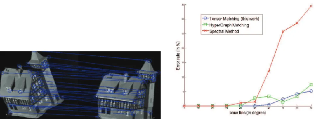
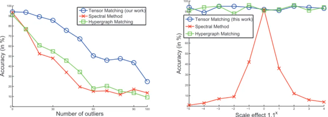
- Synthetic data
- House dataset
- Natural images
- Potentials of different orders
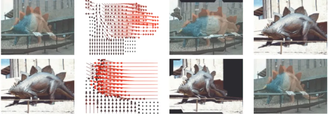
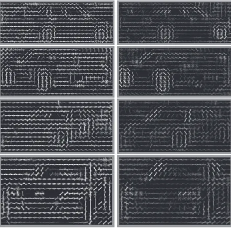
In Figure 2.9 we can see that the low-order algorithms cannot deal with the fact that in perspective transformations the relative positions of points change in a complex way. Using our algorithm, we can then match images from the same class; the results are shown in Figure 2.10. In Figure 2.13.b you can see that the resulting matching is generally correct, but some details are wrong.
Conclusion
Motivation and goals
As explained in the introductory chapter, the advantage of graph matching methods is that they use the spatial relationship between visual features, as opposed to other methods, such as bag of words, which omit this important information. Although graph matching methods saw some success in image categorization (e.g., [Berg et al., 2005a]), they were soon surpassed. We believe this is a key point, as it is the main problem behind the previous points: the slowness of graph matching forces the use of fewer visual features and simpler machine learning techniques.
Organization and contributions
Previous work
Review of literature
Jegou et al., 2010], image retrieval methods based on feature bags can be viewed as voting schemes among local features where Voronoi cells associated with k-means clusters are used to approximate inter-feature distances. Indeed, image representations that enforce a degree of spatial consistency—such as HOG models [Dalal and Triggs, 2005b], spatial pyramids [Lazebnik et al., 2006b] and their variants, e.g. Boureau et al., 2010; Yang et al., 2010] – usually perform better in image classification tasks than pure bags of features.
Caputo’s method
Proposed approach
Image representation
For each node n in G, we also define the feature vector Fn associated with the corresponding image region. The vectors of the coefficients of this sparse decomposition are used as local sparse features. These local sparse features are then summed over larger image areas by taking, for each dimension of the vector of coefficients, the maximum value over the region (max pooling) [Boureau et al., 2010].
Matching two images
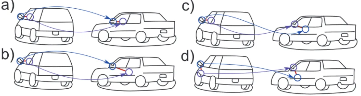
Therefore, we have normalized the descriptions of the images so that the similarity with them has a constant value. In this situation, normalization comes down to dividing an image's descriptors by their ℓ2 norm. Binary potential II: crossing We focus on categorizing objects (as opposed to more general scenes) such that the shape variability for some viewing angles can be represented by image displacements that vary smoothly over the image, and object fragments typically cannot cross each other (see Figure 3.3.c-d ).
A kernel for image comparison
Implementation
Ishikawa’s method
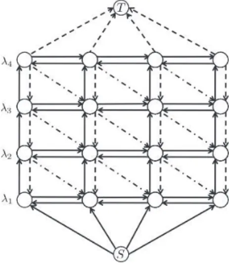
The plain horizontal arrows correspond to the binary potential sum (λj, λj) while the dotted arrows correspond to the non-crossing binary potential vmn(λj, λj −1).
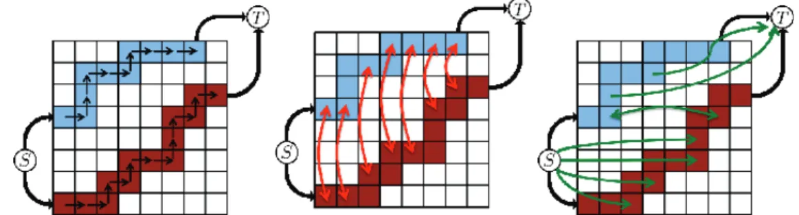
Proposed method: Curve expansion
The blue curve corresponds to nodes(nλb)1≤λ≤Nl obtained by applying labelsλ to the node. A displacement that cannot be related to the corresponding displacements of another node is related to either the sourceS or the sink (best seen in color). An example is shown in Figure 3.6 with two nodes (for test details, see supplementary material).
Experiments
Running time
We use four different strokes (horizontal, vertical and diagonal strokes) to extend the curve in multiple steps. In terms of average minimization performance, 2-step curve expansion is similar to alpha expansion, while 4-stroke multi-step curve expansion and TRW-S improve the results by 2% and 5%, respectively. Thus, the real issue in this context is time, and we prefer to use a two-step curve fitting that matches two images in less than 0.04 seconds for 500 nodes.
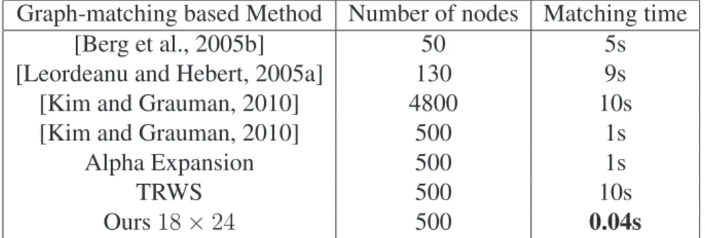
Image matching
Image classification
Conclusion
Motivation and goals
Most modern approaches to visual image interpretation and scene analysis consist of three main components: an image model, a measure of similarity between instances of this model, and a classifier based on it. For example, the pedestrian detector of [Dalal and Triggs, 2005a] uses HOG features as an image model, their inner product as a similarity measure, and a linear SVM in sliding window mode to find people in images. Likewise, the degree of similarity should be invariant to these factors, but able to distinguish between different object classes.
Proposed approach
Image Model
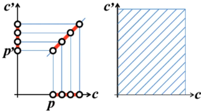
Given cells c and c′ in the first and second images, we define ι(c,c′) as the similarity of the corresponding image descriptors, measured by their dot products. Finally, we can measure the similarity of two bounding fieldbands' as the sum of the similarities of their parts, i.e. As will be shown in the next section, this is the key to very efficient similarity calculations regardless of the depth of the hierarchy.

Efficient Similarity Computation
Changing the values of pandp′ changes where the line segment is located, but not its slope, and if follows that the similarities of any pair of parts can be calculated in constant time using 2D integral images summarizing similarities along diagonal lines . Let's ignore boundary effects (again, for simplicity) and assume that all parts inb andi′ can be moved anywhere in the range D. As mentioned in Section 4.2.1, deeper hierarchies involving several layers of moving parts can be easily accommodated by a simple generalization of the approach presented so far: Similarities between boxes and images can be calculated according to the same scheme, alternating sum and max operations over two-dimensional arrays, and the overall cost remains the optimal cost for a small constant time (see Figure 4.9 for a one-dimensional example).
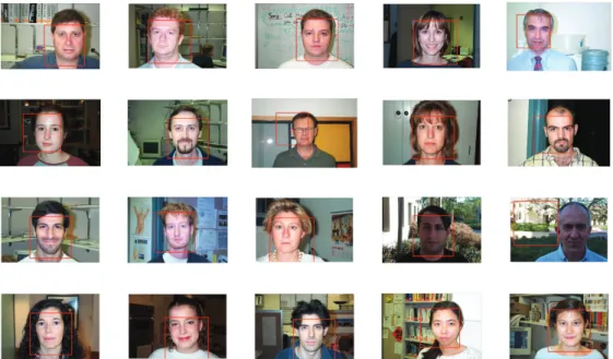
Proof of concept: automated object discovery
As a simple proof of concept (see Figure 4.10), we take some faces from the Caltech2 face dataset. We place the reference bounding box where it maximizes the sum of similarities with other images. Then, we place the other bounding boxes where they maximize their similarity to the reference bounding box.
Learning a detector
Latent SVMs
Hybrid method: Latent SVM and exemplar SVM
We use a very simple optimization scheme: we initialize the template with one positive sample, and then we alternate between (1) computation (for each sample I)ϕ(I, d(wp, I)), (2) optimization of onwp (with libSVM [Chang and Lin, 2001]). The positive examples Ip are images extracted from the positive training boundary blocks plus a large margin. Our similarity measure finds the subimage of Ip that is most similar to T.
Implementation and Results
The next four rows show, for comparison, the results obtained by [Malisiewicz et al., 2011] and [Felzen-szwalb et al., 2010] without and with contextual information. Comparing our results with [Malisiewicz et al., 2011] and [Felzenszwalb et al., 2010] is a little more difficult since we only use a random subset of the data, which can bias things a bit. In general, [Felzenszwalb et al., 2010] dominates the other two methods in our experiments, which may be due to the more sophisticated use of aspect and contextual information.
Conclusion
Note that the contextual model of [Felzenszwalb et al., 2010] is much more powerful than the one used in [Malisiewicz et al., 2011] and our work, as it involves the simultaneous occurrence of multiple classes.
Contributions
Future work
Detection experiments
Since each of them has to be compared to each test image, this leads to a considerable slowdown of our method. Therefore, we will also introduce a combination of our similarity measure with aspects of a latent SVM [Felzenszwalb et al., 2008a] using strain as a latent variable. This way, we would only need to compare a few templates (one per aspect) against each test image, resulting in a significant speedup.
Aspects and full object model
Additionally, each template will use more positive examples for training, which could lead to better generalization.
Joint Alignment of multiple images
Other work
In this appendix we consider the problem of maximizing a convex function on V on a product of ℓ2-spheres of dimension N2, i.e. on the quantity C2. Since havingf(v0) =f(v1) impliesv1 =v0, the sequence also converges and its limitv∞ is such that for eachi1∇f(v∞)i1 is equal to a positive constant timesv∞i1, i.e. v∞ is a stationary point of f on the product of spheresC2 [Absil et al., 2008]. Local features and kernels for classifying texture and object categories: An in-depth study.
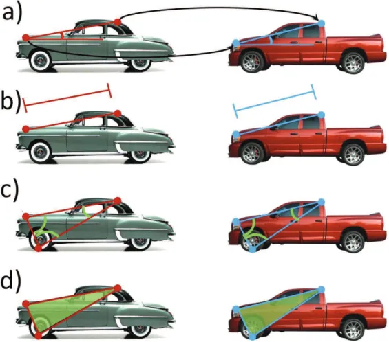
![Figure 1.4: The algorithm of [Huttenlocher and Ullman, 1987a] searches for the prototype (left) in the test image (center) by looking for correspondences, generat-ing transformation hypotheses](https://thumb-eu.123doks.com/thumbv2/1bibliocom/463114.68938/16.892.160.672.357.618/figure-algorithm-huttenlocher-searches-prototype-correspondences-transformation-hypotheses.webp)
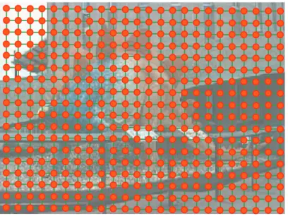
![Figure 1.7: [Lades et al., 1993] align grids on prototypes to test images in order to detect object categories.](https://thumb-eu.123doks.com/thumbv2/1bibliocom/463114.68938/20.892.178.652.476.596/figure-lades-align-prototypes-images-detect-object-categories.webp)
![Figure 1.6: [Yuille, 1991] Hand-designed eye model (deftemplates91). Eye model to eye image alignment (center-left)](https://thumb-eu.123doks.com/thumbv2/1bibliocom/463114.68938/20.892.127.704.187.360/figure-yuille-hand-designed-model-deftemplates91-alignment-center.webp)
![Figure 1.8: [Felzenszwalb et al., 2008b] have produced a state-of-the-art object detector based on a deformable models trained from data](https://thumb-eu.123doks.com/thumbv2/1bibliocom/463114.68938/21.892.212.743.193.436/figure-felzenszwalb-produced-object-detector-deformable-models-trained.webp)