For the purposes of the thesis, we are particularly interested in the infinite horizon problem (T = +∞ and ψ ≡0) and the Bolz problem (T <+∞in λ= 0). The value function is a mapping that associates any initial time t and initial position x with the cost of the optimization problem (1.4).
Hamilton-Jacobi-Bellman Approach
Constrained viscosity solutions
The value function is the finite viscosity solution of the HJB equation, that is, ϑ(·) is a supersolution in K and a subsolution in int(K). This is mainly due to the lack of information on the limits of state restrictions.
Optimal Feedback Laws
Discontinuous ODEs and robustness
In the approach described earlier, the singularities of the feedback do not play any role. On the other hand, the authors in [42] proved that it is possible to construct a suboptimal sample-and-hold feedback that is robust to measurement error, if the partition is chosen appropriately.
Singularities of optimal feedbacks
Question: Can we construct a theory that provides well-posedness for the closed-loop system (1.5) if the singularities of the feedback laws are a stratified set. Question: Can we construct a suboptimal feedback law from an optimal one in such a way that any curve associated with a near-optimal strategy is a suboptimal trajectory of the control system.
Organization of the Manuscript
We emphasize that this last concept is essential to the rest of the present manuscript. On the other hand, invariance theory usually requires a certain regularity of dynamical systems.
Set-valued analysis
Continuity
A set-value map Γ:X ⇒Y is called compact upper semicontinuous atx ∈dom Γ, provided for every compact subset S ⊆Y, the map x7 → Γ(x)∩ S is upper semicontinuous. Let Γ be a top semi-continuous set-value map with closed images and also with closed domΓ.
Selection theorems
Nonsmooth and variational analysis
Elements of convex analysis
The relative interior of S, written ri(S), is the interior of S in the induced topology of its affine hull. In light of the previous theorem, a convex proper and lower semi-continuous function g :X →R∪ {+∞} that is essentially smooth and at the same time essentially strictly convex is called the Legendre function.
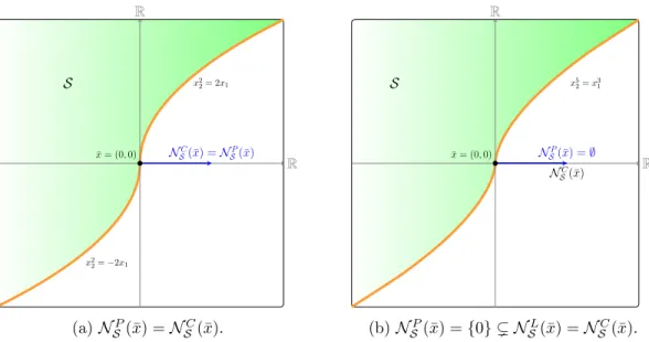
Tangent and normal cones
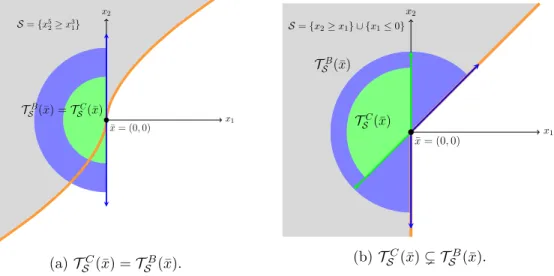
Chapter 2, Section 2.3 Nonsmooth Analysis and Dynamical Systems This cone, viewed as a multifunction, always closed images. In particular, TSC(x) ⊆ TSB(x) for any x ∈ S and equality holds when TSB(·) is lower semi-continuous at x.
Subdifferentials
Non-smooth and analysis of variations Chapter 2, Section 2.3 Throughout this section, ω(·) stands for lower semi-continuous functions defined onX with values in R∪ {+∞} whose effective domain is not empty. The following is a well-known formula that is verified when ω:X →R∪ {+∞} is a convex lower semicontinuous function.
Differential inclusions
Existence of solutions
In this case, the existence of a solution remains valid, provided that the dynamics have non-empty, convex, and compact images. This is a direct consequence of the convergence theorem, the statement of which we have adapted to the current framework.
Invariance of dynamical systems
This proposition is similar in spirit to Theorem 4.1 in [17] and is an extension of the classical criterion for strong invariance found in the current literature; EG In this dissertation we deal with well-structured state constraints and feedback controls, in particular, in the case where a layering of the state space can be associated with one of the aforementioned objects.
Notation
This has been reported in Section 3.4 and in [67], which makes the content of this section new and can be considered part of the contribution to the thesis. The rest of the results are part of the thesis contribution, and as mentioned before, most of them have been reported in [66, 67] or are under consideration for future publications.
Embedded Manifolds
An alternative definition
In a much more abstract setting, instead of a vector space, we could consider embedded manifolds of a given smooth manifold. Chapter 3, Section 3.2 Manifolds and Stratifications The smooth structure of the Ck-smooth manifold allows the classical notions of differentiability to be extended to this context in the manner described below.
Tangent and normal spaces
Chapter 3, Section 3.2 Manifolds and stratifications The fact that the tangent space can be interpreted as the kernel of a matrix also suggests that the map x 7→ TM(x) can be quite regular as a set-valued map, but it are rarely continuous. The previous result shows that the tangent space is rarely locally Lipschitz continuous, even if the manifold is highly differentiable.
Differentiable functions and extensions
In particular, (3.1) is still valid (L could be larger) if the infimum is adopted Γ(ˆx) instead of TM(ˆx). Chapter 3, Section 3.3 Manifolds and Stratifications On the other hand, let {ϕx}x∈M be a C∞ partition of the unit subordinate to the set {BX(x, rx)}x∈M, which is an open covering of M ; we refer to [3, Theorem 3.14].
Stratifications
Whitney regularity conditions
The significance of Whitney's (b)-condition is that, contrary to (a)-condition, any pre-stratification that satisfies it is a stratification. Despite the fact that Whitney's (b)-condition always implies Whitney's (a)-condition, the latter is sufficient for the purposes of the following explanations, as we shall see later.
Some favorable classes of stratifiable sets
If by Saln we denote the set of all semialgebraic subsets of Rn, then Sal:={Saln}n∈N is an o-minimal structure (actually the smaller possible). On the other hand, another important type of sets that can be seen as elements of an o-minimal structure are the so-called finitely subanalytic sets.
Normals and tangents
By virtue of the Whitney (a) condition applied to (Mi,Mk), one gets that TMi(x)⊆ T and in particular η ∈ NMi(x). The above statement has a very interesting consequence regarding the regularity of the Clarke cones to layer closure.
Relative wedgedness
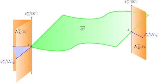
Chapter 3, Section 3.4 Manifolds and Layers Furthermore, given that the structure of cones essentially relies on the local group structure, TMCi(x) = TMi(x) and NMi(x) = NMCi(x) for every x ∈ Mi; this is thanks to Propositions 3.2.2 and 3.2.3, respectively. The utility of the projection is reflected in the following statement, which describes in particular the relative interior of the Clarke tangent cone.
Discussion and perspectives
In this section, we address the question of how to characterize the value function of an optimal state-constrained control process in terms of a Hamilton-Jacobi-Bellman equation. In this chapter, we present an approach to study the value function of an optimal control problem with stratifiable state constraints.
Introduction
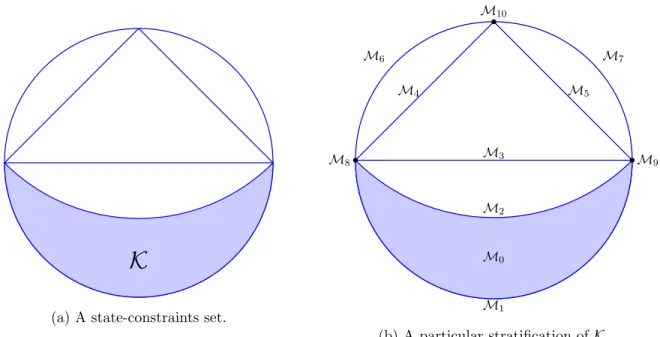
Stratifiable state-constraints
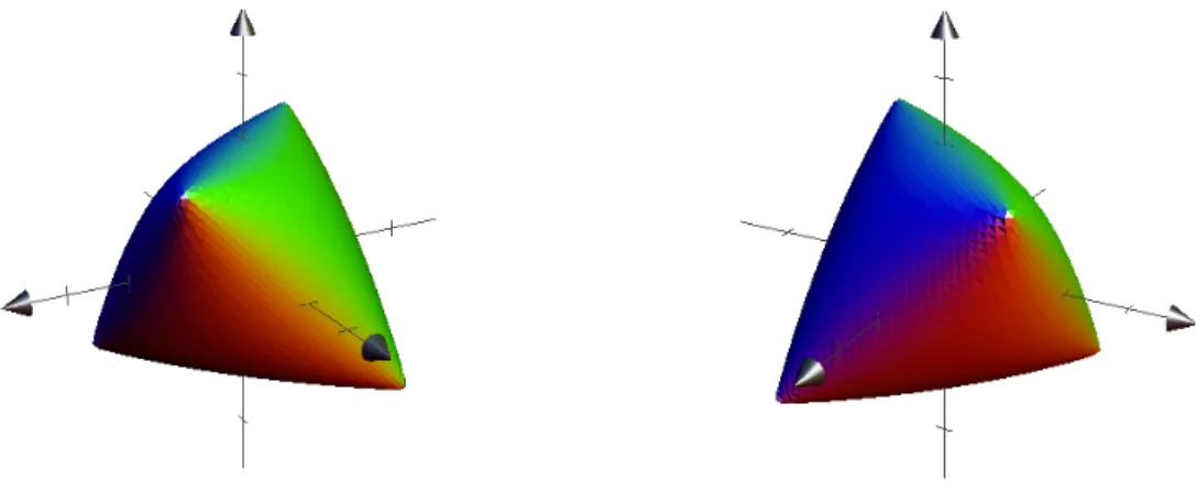
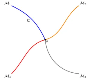
One of the first and simpler is when K is a closed manifold (compact manifold without boundary); the torus embedded in R3, illustrated in Figure 4.1, is a good model. More general networks can also be considered as in Figure 4.3b where the collection K is a network embedded in the space R3.

Infinite horizon problems
Compatibility assumptions
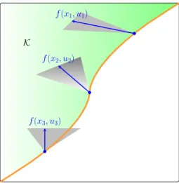
Then the map with set values of the tangent to Mi for every i∈ I has compact images and is uppermost semi-continuous at Mi. Consequently, by the continuity of the dynamics, we get f(xn, un) →f(x, u) and since f(xn, un)∈ TMi(xn), the multifunctional Ai is uppermost semi-continuous on Mi.
Characterization of the Value Function
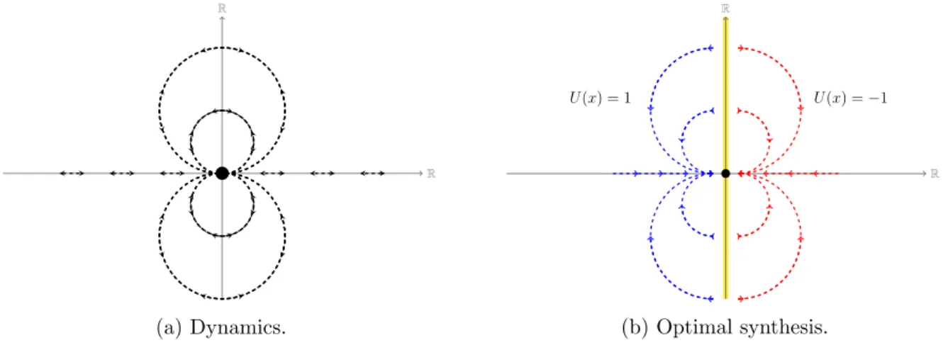
Therefore, adapting the classical arguments to this setting, we can see that (4.6) implies the Lipschitz regularity of the minimal time function of the controlled dynamics bounded on the multiple Mi, and thus (H34) follows; c.f. For example, the controlled harmonic oscillator system in Example 4.2.1 satisfies the requirement (H34) and clearly does not satisfy the Petrov condition (4.6); this is mainly due to the fact that the controllability hypothesis is only relevant around layers M3 and M4 (otherwise it is straightforward) which are the trajectories of the system themselves.
Proof of the main result
Therefore, by the monotonic convergence theorem, (4.12) and the definition of the value function, we obtain the desired inequality ϑ(x)≤ϕ(x). In light of the previous lemma, the necessity part of the strongly increasing principle can be stated as follows.
Application to networks
In the rest of the section, we will assume that Ki is a closed network on RN. Using this adapted version of the weakly descending principle, we obtain the following characterization of the value function in networks.
Mayer problems
The Value Function and compatibility assumptions
Then the value function of the Mayer problem is the unique lower semicontinuous function on [0, T]× K which is +∞ outside [0, T]× K and which verifies . We evoke that the value function of the Mayer problem solves the functional equation ϑ(t, x) = inf.
Decreasing principle
The previous lemma leads to the claim, as in Proposition 4.2.4, that the value function is a unique function that is slightly decreasing and at the same time strongly increasing along ST trajectories. Therefore, it only remains to show that ϕ falling slightly along the ST trajectories means that (4.34) holds.
Increasing principle
This statement is the corresponding version of Step 2 in the proof of Proposition 4.2.7, and the idea of the proof is similar. To summarize, we have constructed a trajectory of control systems for which the set {s∈[t, Tε]|yε(s)∈ Mi} can be decomposed into a finite number of intervals.
Discussion and perspectives
- Contributions of the chapter
- Optimality principles
- Lipschitz-like hypothesis
- Convex sets
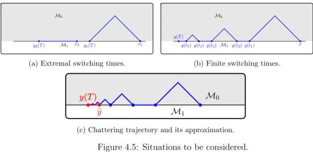
The characterization of the value function can then be considered in terms of bilateral viscosity. For any control system trajectory y(·) with initial condition (t) =x and any T > t, we can find ˜T > t as close as desired from T and a non-talking curve of control systems ˜ y( ·) with initial condition ˜y(t) =xwhich verifies y(T) = ˜y( ˜T).
Infinite horizon problem and linear systems
Linear systems
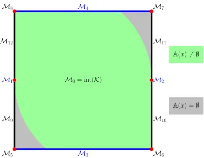
Furthermore, under these conditions, we have that the minimal cost can be approximated by a series of trajectories that most of the time stay on the relative interior of the state constraints. Consider yε = ˜εx0+ (1−ε)¯˜y, this is an absolutely continuous function that remains on ri(K) due to the Accessibility Lemma.
Characterization of the Value Function
In particular, given that ri(K) can be treated as an embedded manifold (Proposition 5.1.1), adapted to the arguments in Section 4.2, it is not difficult to see that ϑ(·) is lower semicontinuous, has λ`-superlinear and verifies (5.2) and (5.3). Then we write yn for yxunn, and thus, in view of the previous remark, for any t >0 we have.
Mayer problem and convex dynamics
Interior approximations
Note that yε is an absolutely continuous function, and by (H25) and the accessibility lemma (Proposition 2.3.1), yε(s)∈ri(K) for any s∈(t, T). In light of the above result, we can give an account analogous to Proposition 5.2.1, adapted to the Mayer problem.
The Value Function
Discussion and perspectives
Contributions of the chapter
End-point constraints and star-shaped sets
We provide a characterization of the value function by means of the Hamilton-Jacobi-Bellman approach. Under this framework we can characterize the value function of the Mayer problem as a unique (continuous) viscosity solution of the Hamilton-Jacobi-Bellman (HJB) equation.
Characterization for the Mayer problem
Chapter 6, Section 6.3 Convex state constraints II: Absorbing dynamics The main theorem we study deals with the characterization of the Value function with convex state constraints for a system where no wise qualification assumption holds. The framework of the problem is set under rather non-standard hypotheses, which are in any case suitable for the penalization technique; the underlying reason is that (H06) allows us to assign Ω with the structure of Riemann manifold.
Dual optimal control problem
The importance of the previous statement lies in the fact that for optimal control problems without state constraints, the Value function can be characterized using the HJB approach. Finally, since the auxiliary problem has no state constraints, it is a classical result that under these circumstances the value function is the unique continuous viscosity solution of the HJB equation on the statement; see for example [13, Theorem 4.7.10] or [129, Theorem 12.3.7].
Auxiliary problem and final proof
Properties of the auxiliary problem
When two functions α and β are defined as above, one can expect differentiation properties of the primary function to be inherited by the dual function and vice versa.
Proof of Theorem 6.2.1
Chapter 6, Section 6.5 Convex State Limits II: Absorption Dynamics The previous arguments show that the value function ϑ is the viscosity solution of the HJB equation on (0, T) × Ω.
Discussion and perspectives
A Riemannian manifolds interpretation
In light of the previous definition, we can see that in this chapter we have actually studied a Mayer problem on a quadratic Hessian Riemann manifold. Actually, the assumption domg∗ = X means nothing else than the completeness of the Riemannian manifold as a metric space endowed with the distance.
Introduction
The main problems are the existence of solutions and the robustness of trajectories with respect to external disturbances on the speed. Particular attention is paid to the interplay between regularity conditions on the quantities Mi and pointwise conditions on the vector field to ensure the existence of solutions.
Stratified vector fields
Stratified ordinary differential equations
For all purposes, (D) is called the stratified ordinary differential equation associated with the stratification {Mi}i∈I and with the dynamics G = {gi : Mi → TMi}i∈I0. It may be that the limiting trajectory lies on Mi for a set of times of positive measure, but this is not a stratified solution.
Existence of stratified solutions
This means that for every tn % T, the sequence {y(tn)} satisfies the Cauchy condition, and hence, the limit is well defined. Using the same inequality, it is possible to prove that the limit does not depend on the obtained sequence.
Moreover, from Corollary 3.3.1 we have that if the stratification satisfies the Whitney (a) condition, x 7→ TMCj(x) is lower semicontinuous for every index j ∈ I, and then, in view of Proposition 3.4.5, the next statement is a direct consequence of the cited results. Furthermore, if the dimension of Mj in (H70) happens to coincide with the dimension of the surrounding space, that is N, relative wedgedness implies that Mj is epi-Lipschitz around x (it is also referred to as wedged sets); c.f [112, section 9.F] and [40, section 3.6].
Necessary condition for Robustness
- Robustness with respect to external perturbations
- Outward-pointing modulus
- The externally perturbed model
- Robustness result
- Proof of Theorem 7.4.1
A Necessary Condition for Robustness Chapter 7, Section 7.4 Then the bound on the magnitude of the perturbation is given by . A similar lemma can be stated if the sign of the outward facing module is negative.
Discussion and perspectives
Contributions of the chapter
Furthermore, the introduction of an outward-directed modulus, as seen in the analysis, provides a practical way to measure the maximum perturbation magnitude and also to identify some favorable classes of singularities that make the system stable with respect to external perturbations. To summarize, the main contribution of the theory that we have recently presented is the possibility of using only the initial data of the problem to determine whether a discontinuous ordinary differential equation admits classical solutions and whether it is stable to external disturbances.
Some extensions
In this chapter we address the question of the construction of a continuous suboptimal feedback from an optimal synthesis. To this end, as done in Chapter 7, we assume that the set of singularities of the feedback admits a stratified structure.
Setting of the problem
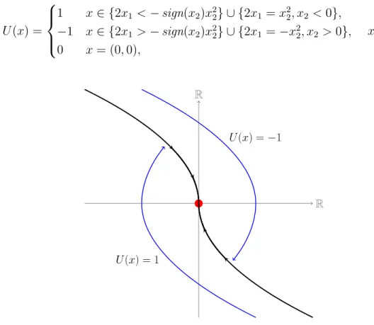
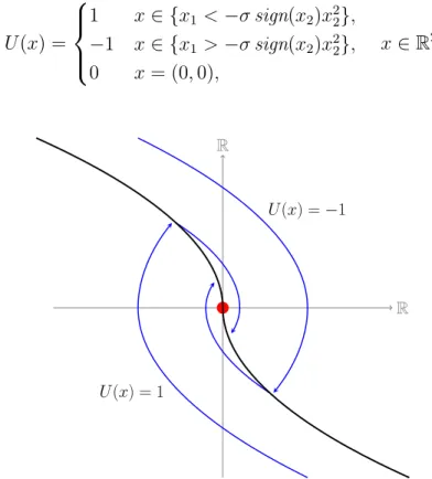
An example: the soft landing problem
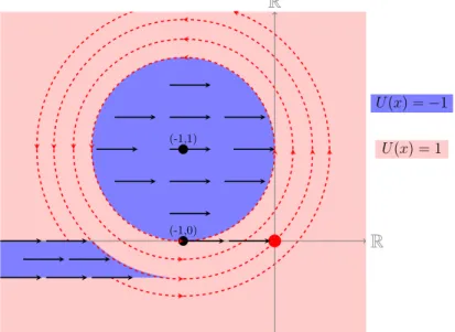
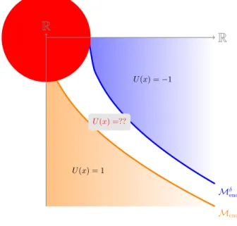
In Figure 8.3, this set is represented by the black curve and the red ball is the ε neighborhood of the origin that we want to reach. Setting up the problem Chapter 8, Section 8.2 We recall that in this situation, the minimum time function to reach the origin can be calculated explicitly and is given by
Control-affine systems
Technical lemmas
Recall that the minimum time function is the classical solution of the Hamilton-Jacobi-Bellman equation on Mini, and so. In particular, given the optimality of the feedback Uend and due to ω, the test function (ω≡TΘ on Mini∪ Mend) we have.
Proof of the principal theorem
In particular, due to the continuity of the vector fields and the fact that f(y(τ), Uend(y(τ)))∈int(TΣC˜r,σ(y(τ))) we can conclude that . Suboptimality of the feedback: Note that TΘ is differentiable along the arc t 7→ y(t) and thus, in view of the control-affine structure of the dynamics, for any t∈(0, τ).
Discussion and perspectives
Contributions of the chapter
Further extensions
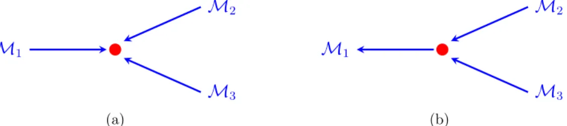
In this chapter, we study optimal control problems on networks without the assumption of controllability at junctions. We are currently working on the Hamilton-Jacobi-Bellman (HJB) approach to control problems in networks.
Setting of the problem
The Mayer problem on networks
This study will be discussed in more detail at the end of the chapter. Problem Statement Chapter 9, Section 9.2 Consequently, the dynamic constraint of the control system is written as follows.
Structural assumptions
Chapter 9, Section 9.2 The HJB approach to optimal convexity control of network dynamics along the constraint set. However, since the main difficulties are mainly at the intersections, it is not difficult to provide some criteria for the stability of the network.
Characterization of the Value Function
A generalized notion of d-dimensional network
Basic definitions and main hypotheses
Characterization of the Value Function
Discussion and perpectives
Junction conditions
Necessary conditions
Generalized networks