HAL Id: hal-01570853
https://hal.inria.fr/hal-01570853v2
Preprint submitted on 18 Aug 2017 (v2), last revised 12 Jul 2018 (v4)
HAL is a multi-disciplinary open access archive for the deposit and dissemination of sci- entific research documents, whether they are pub- lished or not. The documents may come from teaching and research institutions in France or abroad, or from public or private research centers.
L’archive ouverte pluridisciplinaire HAL, est destinée au dépôt et à la diffusion de documents scientifiques de niveau recherche, publiés ou non, émanant des établissements d’enseignement et de recherche français ou étrangers, des laboratoires publics ou privés.
orthogonal group
Paul Görlach, Evelyne Hubert, Théo Papadopoulo
To cite this version:
Paul Görlach, Evelyne Hubert, Théo Papadopoulo. Rational invariants of ternary forms under the orthogonal group. 2017. �hal-01570853v2�
UNDER THE ORTHOGONAL GROUP
PAUL GÖRLACH, EVELYNE HUBERT, AND THÉO PAPADOPOULO
Abstract. In this article we determine a generating set of rational invariants of minimal cardinality for the action of the orthogonal group O3 on the spaceR[x, y, z]2d of ternary forms of even degree 2d. The construction relies on two key ingredients: On one hand, the Slice Lemma allows us to reduce the problem to dermining the invariants for the action on a subspace of the finite subgroup B3of signed permutations.
On the other hand, our construction relies in a fundamental way on specific bases of harmonic polynomials.
These bases provide maps with prescribed B3-equivariance properties. Our explicit construction of these bases should be relevant well beyond the scope of this paper. The expression of the B3-invariants can then be given in a compact form as the composition of two equivariant maps. Instead of providing (cumbersome) explicit expressions for the O3-invariants, we provide efficient algorithms for their evaluation and rewriting.
We also use the constructed B3-invariants to determine the O3-orbit locus and provide an algorithm for the inverse problem of finding an element inR[x, y, z]2dwith prescribed values for its invariants. These are the computational issues relevant in brain imaging.
Contents
1. Introduction 1
2. Preliminaries 6
3. The Slice Method 10
4. Invariants of ternary quartics 13
5. Harmonic bases with B3-symmetries and invariants for higher degree 18
6. Solving the main algorithmic challenges 28
References 32
1. Introduction
Invariants allow to classify objects up to the action of a group of transformations. In this article we determine a set of generating rational invariants of minimal cardinality for the action of the orthogonal group O3 on the spaceR[x, y, z]2d of ternary forms of even degree 2d. We do not give the explicit expression for these invariants, but provide an algorithmic way of evaluating them for any ternary form.
Classical Invariant Theory [GY10] is centered around the action of the general linear group on homogeneous polynomials, with an emphasis on binary forms. Yet, the orthogonal group arises in applications as the relevant group of transformations, especially in three-dimensional space. Its relevance to brain imaging is the original motivation for the present article.
Computational Invariant Theory [DK02, GY10, Stu08] has long focused on polynomial invariants. In the case of the group O3, any two real orbits are separated by a generating set of polynomial invariants. The generating set can nonetheless be very large. For instance a generating set of 64 polynomial invariants for the action of O3onR[x, y, z]4 is determined as a subset of a minimal generating set of polynomial invariants of the action of O3on theelasticity tensor in [OKA17]. There, the problem is mapped to the joint action of
Date: August 18, 2017.
SL2(C) on binary forms of different degrees and resolved by Gordan’s algorithm [GY10, Oli16] so that the invariants are given as transvectants.
A generating set of rational invariants separates general orbits – this remains true for any groups, even for non-reductive groups. Rational invariants can thus prove to be sufficient, and sometimes more relevant, in applications [HL12, HL13, HL16] and in connection with other mathematical disciplines [HK07b, Hub12].
A practical and very general algorithm to compute a generating set of these first appeared in [HK07a]; see also [DK15]. The case of the action of O3 on R[x, y, z]4, a 15-dimensional space, is nonetheless not easily tractable by this algorithm. In the case ofR[x, y, z]4, the 12 generating invariants we construct in this article are seen as being uniquely determined by their restrictions to a slice Λ4, which is here a 12-dimensional subspace. The knowledge of these restrictions is proved to be sufficient to evaluate the invariants at any point in the spaceR[x, y, z]4. The systematic computational use of characterization of invariants in terms of their restrictions to aslice is a novel approach to Computational Invariant Theory that we shall introduce.
More generally, by virtue of the so-called Slice Lemma, the field of rational invariants of the action of O3
on R[x, y, z]2d is isomorphic to the field of rational invariants for the action of the finite subgroup B3 of signed permutations on a subspace Λ2d of R[x, y, z]2d. Working with this isomorphism, we provide efficient algorithms for the evaluation of a (minimal) generating set of O3invariants based on a (minimal) generating set of B3-invariants. Finding an element ofR[x, y, z]2d with prescribed values of O3-invariants and rewriting any O3-invariant in terms of the generating set are also made possible through the specific generating sets of B3-invariants we construct.
R[x, y, z]2d decomposes into a direct sum of O3-invariant vector spaces determined by the harmonic poly- nomials of degree 2d,2d−2, . . . ,2,0. The construction of the B3-invariants relies in a fundamental way on specific bases of harmonic polynomials. These bases provide maps with prescribed B3-equivariance proper- ties. Our explicit construction of these bases should be relevant well beyond the scope of this paper. The explicit expression of the B3-invariants can then be given in a compact form as the composition of two equivariant maps. Both the rewriting and the inverse problem can be made explicit for this well-structured set of invariants.
The whole construction is first made explicit forR[x, y, z]4 and then extended toR[x, y, z]2d. It should then be clear how one can obtain the rational invariants of the joint action of O3on similar spaces, as for instance the integrity tensor.
In the rest of this section we first introduce the geometrical motivation and then the context of application for our constructions around the invariants of the action of O3 onR[x, y, z]2d. Notations, preliminary material and a formal statement of the problems appear then in Section 2. In Section 3, we describe the technique for reducing the construction of invariants for the action of O3 onR[x, y, z]2d to the one for the action of a finite subgroup, the signed symmetric group, on a subspace. Based on this, we construct a generating set of rational invariants for the case of ternary quartic forms in Section 4. We extend this approach in Section 5 to ternary forms of arbitrary even degree; central there is the construction of bases of vector spaces of harmonic polynomial with specific equivariant properties with respect to the signed symmetric group. Finally, we solve the principal algorithmic problems associated with rational invariants in Section 6.
1.1. Motivation: spherical functions up to rotation. In geometric terms, the results in this paper allow to determine when two general centrally symmetric closed surfaces inR3 differ only by a rotation.
The surfaces we consider are given by a continuous functionf: S2→Ron the unit sphere S2:={(x, y, z)∈ R3|x2+y2+z2= 1}. The surface is then defined as the set of points
S:={(x f(x, y, z), y f(x, y, z), z f(x, y, z))∈R3|(x, y, z)∈S2} ⊂R3,
i.e. for each point on the unit sphere we rescale its distance to the origin according to the functionf. For example, the surface described by a constant functionf ≡r (for somer∈R) is the sphere with radius |r|
centered at the origin. As f takes on more general functions, a large variety of different surfaces can be described. For the surface to be symmetric with respect to the origin, one needs the function f to satisfy
Figure 1.1. Two centrally symmetric surfaces only differing by a rotation.
the property
(1.1) f(p) =f(−p) ∀p∈S2.
Since the unit sphere S2⊂R3is a compact set, the Stone–Weierstraß Theorem implies that a given continuous function S2→Rcan be approximated arbitrarily well by polynomial functions, i.e. by functions f:S2→R of the form
(1.2) f(x, y, z) = X
i+j+k≤d
aijkxiyjzk.
The symmetry property (1.1) is then fulfilled if and onlyaijk= 0 wheneveri+j+kis odd, in other words, f must only consist of even-degree terms. We can then rewrite f in such a way that all its monomials are of the same degree, by multiplying monomials of small degree with a suitable power ofx2+y2+z2(which does not change the values off sincex2+y2+z2= 1 for all points (x, y, z) on the sphere).
We therefore model closed surfaces that are centrally symmetric with respect to the origin byf: S2→R, a polynomial function of degree 2d:
f(x, y, z) = X
i+j+k=2d
aijkxiyjzk.
The modeled surface can then be encodedexactlyby simply storing the 12(2d+ 2)(2d+ 1) numbersaijk∈R. However, from such an encoding of a surface via the coefficients aijk of its defining polynomial, it is not immediately apparent when the defined surfaces have the same geometric shape, only differing by a rotation.
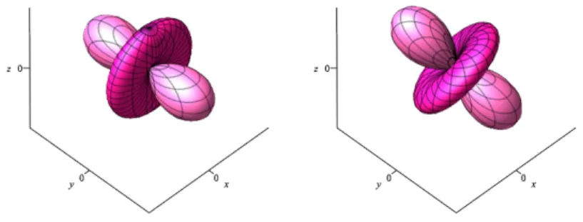
As an example, Figure 1.1 depicts the two surfacesS1andS2described by f1(x, y, z) := 18x2−27y2+ 18z2 and
f2(x, y, z) := 13x2+ 20xy−20xz−2y2+ 40yz−2z2,
respectively, whose numerical description in terms of coefficients look very distinct, but whose shapes look very similar. IndeedS2 arises fromS1 by applying the rotation determined by the matrix
1 3
2 −1 −2
2 2 1
1 −2 2
,
so that
f2(x, y, z) =f1
2x+ 2y+z
3 ,−x+ 2y−2z
3 ,−2x+y−2z 3
.
In general, we want to consider surfaces to be of the same shape if they differ by a rotation or, equivalently, by an orthogonal transformation: Since we only consider surfaces symmetric with respect to the origin, two surfaces differing by an orthogonal transformation also differ by a rotation.
The question which arises is: How can we (algorithmically) decide whether two surfaces only differ by an orthogonal transformation, only by examining the coefficients of their defining polynomial?
Regarding this question, we should to be aware that if f: S2→R describesS ⊂ R3, then its negative−f describes the same setS ⊂ R3. With the intuition of describing the surface by deforming the unit sphere, this ambiguity corresponds to turning the closed surface S inside out. We typically want to think of the surfaces defined byf and by−f as two distinct objects (even though they are equal as subsets ofR2). For example, the surface defined by the constant functionf ≡1 is the unit sphere, while the surface defined by f ≡ −1 should be considered as the unit sphere turned inside out.
Then the question above corresponds to the following algebraic question:
Question 1.1. Given two polynomials f =P
i+j+k=2daijkxiyjzk and g=P
i+j+k=2dbijkxiyjzk, how can we decide in terms of their coefficientsaijk andbijk whether or not there exists an orthogonal transformation ϕ: R3→R3 such that f =g◦ϕas functionsR3→R?
Once we can decide whether two polynomials define equally shaped surfaces, a natural question is how to uniquely encode the shape of a surface, i.e. an equivalence class of surfaces up to orthogonal transformations.
The corresponding question for polynomials is:
Question 1.2. How can we encode in a unique way equivalence classes of polynomials up to orthogonal transformations?
For the purpose of illustration we discuss next the case of homogeneous polynomials of degree two, i.e.qua- dratic forms. In the following section, we shall describe the mathematical setup for addressing Questions 1.1 and 1.2 with the rational invariants of the action of the orthogonal group on ternary forms of even degree.
Illustration for the case of quadratic surfaces. Quadratic forms are in one-to-one correspondence with sym- metric 3×3-matrices, as indeed we can write (1.2) as:
(1.3) f(x, y, z) = x y z
a200 1
2a110 1 2a101 1
2a110 a020 1 2a011 1
2a101 1
2a011 a002
| {z }
=:A
x y z
When we composef with a rotation, given by a matrixR, we obtain another homogeneous polynomial of degree 2. The defining symmetric matrix (as in 1.3) of the obtained polynomial is then RART. For two symmetric matrices Aand B, Linear Algebra then tells us that there is an orthogonal matrix Rsuch that B =RART if and only if Aand B have the same eigenvalues. Yet, eigenvalues are algebraic functions of the entries of a matrix and thus cannot be easily expressed symbolically. It is thus easier to compare the coefficients of the characteristic polynomials. Up to scalar factors, these are:
(1.4)
e1:=a200+a020+a002,
e2:= 4a020a200+ 4a002a020+ 4a002a200−a2110−a2101−a2011, e3:= 4a002a020a200+a101a110a011−a2101a020−a2011a200−a002a2110.
The result is that two homogeneous polynomial of degree 2 are obtained from one another by an orthogonal transformation if and only if the functionse1, e2, e3 of their coefficients take the same values. This answers Question 1.1 in this case. The functionse1, e2, e3also provide a solution to Question 1.2. To each polynomial of degree 2 we can associate a point in R3 whose components are the values of the functions e1, e2, e3 for this polynomial. All equivalent polynomials will be mapped to the same point. One can check for example that this point is (9,−2592,−34992) for both f1 andf2 defined above.
1.2. Application in Neuroimaging. DMRI (Diffusion Magnetic Resonance Imaging), developed since 1984, is a field where the problem of characterizing spherical shapes arises. DMRI measures non-invasively the amount of water diffusion in biological tissues. These diffusion properties are intimately related to the
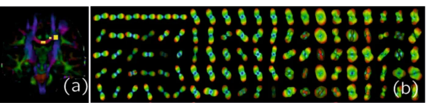
Figure 1.2. Slice of a brain diffusion image (a). The yellow boxes indicate the regions that are zoomed in (b) showing the individual voxel shapes. From [PGD14].
structure of these tissues notably in fibrous structures such as muscles – e.g. the heart – or brain white matter.
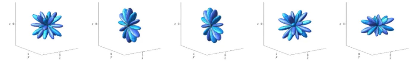
The measurements are made in a rectangular portion of the 3D space sampled by voxels (volumic picture element). At each voxel, the diffusion information is captured as a function f: S2 → R≥0 of orientation v, sampled at several points vi on the sphere S2. This (discretized) spherical function f is called an ODF (diffusion Orientation Distribution Function) [TRWW03]. Here f(v), for v ∈ S2, is a positive value that characterizes the amount of diffusion in the direction v in a given amount of timeT (which is a constant defined in the diffusion acquisition protocol). f satisfies f(v) =f(−v), meaning thatf is symmetric with respect to the origin. Figure 1.2 shows an example of such a diffusion image for brain white matter.
Integrating the discrete diffusion information into a global model is interesting for e.g. noise reduction or for computing mathematical properties off. This global model was initially a simple a ternary quadratic function (or tensor), leading to what is called Diffusion Tensor Imaging (DTI). For DTI, all rotational invariants can be easily computed as functions of e1, e2, e3 given in (1.4). Biologically interesting quanti- ties have been computed as combination of these invariants, with clinical validation showing their interest to detect various important deseases such as Alzheimer’s or Parkinson’s diseases, writer’s cramp disease, etc [DVW+09, LMM+10].
With diffusion MRI improvements, acquiring more and more samples on the sphere S2 is both possible and interesting (High Angular Resolution Diffusion-weighted Imaging - HARDI - technique [Tuc02]). This allows the study of complex fibrous structures, e.g. revealing places in the brain where white matter fiber bundles are crossing, with the potential of characterizing more completely such complex structures and their abnormalities which may occur in patients. Fully exploiting these images can only be realized using shapes for the diffusion information more complex than those described by quadratic forms.
One popular solution is to representf using a spherical harmonic basis [Fra02]. Because of the symmetry property mentioned above, only spherical harmonics of even order are meaningful. Using spherical harmonic functions up to order 2d is mathematically equivalent to representing f as a homogeneous polynomials of even degree 2d:
f(x, y, z) = X
i+j+k=2d
aijkxiyjzk.
Of particular interest is the case of degree 2d= 4 introduced in [BVF08] as it is the simplest model generaliz- ing the DTI case (2d= 2) and as the positivity off can be imposed using Hilbert’s ternary quartic theorem.
Since then, numerous efforts have been made to obtain a complete invariant description for these homoge- neous polynomials of degree 2d= 4 [BP07, GPD12a, GPD12b], with the prospect of finding more powerful generalizations of the biomarkers found in the DTI case. A maximal set of functionally independent local invariants were proposed in [PGD14]; they are algebraic functions of aijk ∈R. Functionally independent sets of polynomial invariants were also determined in [CV15] for the cases 2d= 4 and 2d= 6.
The present article provides a complete (functionally independent and generating) set of rational invariants, for all even degrees 2d.
2. Preliminaries
In order to set the notation, we review the definitions of the action of O3 on the vector space of forms Vd:=R[x, y, z]d and of its rational invariants. We then elaborate on the Harmonic Decomposition ofV2d. 2.1. The action of the orthogonal group on homogeneous polynomials. We start out with a few notational conventions. We denote byR[x, y, z]d the set of homogeneous polynomials
f = X
i+j+k=d
aijkxiyjzk
of degreedin the three variablesx, y, zwith real coefficientsaijk ∈R. By O3⊂R3×3 we denote the group of orthogonal matrices and we consider the action of O3 onR[x, y, z] given by
O3×R[x, y, z]d → R[x, y, z]d
(g, f) 7→ f◦g−1.
By f◦g−1, we mean the composition of the orthogonal transformationg−1:R3→R3 with the polynomial functionf:R3→R, resulting in a different polynomial function that we denote bygf. Note thatgf is again homogeneous of degreed, so the above action is well-defined. Asg−1=gT, the polynomialgf is obtained fromf by applying the substitutions
x7→g11x+g21y+g31z, y7→g12x+g22y+g32z, z7→g13x+g23y+g33z,
when g = (gij) ∈ O3 is an orthogonal 3×3-matrix with entries gij. The use of the inverse g−1 (= gT) instead ofg in the above composition is only of notational importance, guaranteeing g1(g2f) = (g1g2)f for allg1, g2∈O3.
A counting argument shows that there areN := d+22
=12(d+ 2)(d+ 1) monomialsxiyjzk of degreed, so formally,R[x, y, z]d is anN-dimensional vector space overR. In order to stress this point of view, we shall denote
Vd:=R[x, y, z]d
and, accordingly, we shall from now on typically denote elements ofVdby letters likevorw. The monomials {xiyjzk | i+j+k =d} form a basis for this vector space. But alternative bases will prove useful in this paper.
Asg(v+w) =gv+gwandg(λv) =λ(gv) holds for allg∈O3,v, w∈Vd andλ∈R, the action of O3 onVd
is alinear group action. If we fix a basis forVd, there is polynomial map from O3to the group of invertible N×N matrices that describes the action of O3onVd in this basis.
Example 2.1 (The action on quadratic forms). We show the matrix that provides the transformation by g= (gij)1≤i,j≤3∈O3 onV2in two different bases, starting with the monomial basis.
If
f :=a200x2+a110xy+a020y2+a101xz+a011yz+a002z2 and
gf =b200x2+b110xy+b020y2+b101xz+b011yz+b002z2, then the relation between the coefficients off andgf is given by the matricial equality:
b200
b110
b020
b101
b011
b002
=
g211 g11g12 g122 g11g13 g12g13 g213 2g21g11 g21g12+g11g22 2g22g12 g21g13+g11g23 g22g13+g12g23 2g23g13
g221 g21g22 g222 g21g23 g22g23 g223 2g31g11 g31g12+g11g32 2g32g12 g31g13+g11g33 g32g13+g12g33 2g33g13
2g31g21 g31g22+g21g32 2g32g22 g31g23+g21g33 g23g32+g22g33 2g33g23
g231 g31g32 g322 g31g33 g32g33 g233
a200
a110
a020
a101
a011
a002
Let us denote byR(g) the matrix in the above equality.
Alternatively the set of polynomials{x2+y2+z2, yz, zx, xy, y2−z2, z2−x2}forms a basis forV2. LetP be the matrix of change of basis, i.e.
x2+y2+z2 yz zx xy y2−z2 z2−x2
= x2 xy y2 zx yz z2 P If
f =a1(x2+y2+z2) +a2yz+a3zx+a4xy+a5(y2−z2) +a6(z2−x2) and
gf =b1(x2+y2+z2) +b2yz+b3zx+b4xy+b5(y2−z2) +b6(z2−x2), then the vector of coefficientsb= b1 . . . b6T
is related to the vector of coefficientsa= a1 . . . a6T
by the matricial equality:
b= ˜R(g)a, where ˜R(g) =P−1R(g)P Using thatg∈O3, one can compute that
R(g) =˜
1 0 0 0 0 0
0 g23g32+g22g33 g31g23+g21g33 g31g22+g21g32 2g32g22−2g33g23 2g33g23−2g31g21
0 g32g13+g12g33 g31g13+g11g33 g31g12+g11g32 2g32g12−2g33g13 2g33g13−2g31g11
0 g22g13+g12g23 g21g13+g11g23 g21g12+g11g22 2g22g12−2g23g13 2g23g13−2g21g11
0 g22g23 g21g23 g21g22 g222 −g223 g232 −g212
0 g32g33+g22g23 g31g33+g21g23 g31g32+g21g22 g222 +g322 −g223−g233 g232 +g332 −g212 −g231
.
Hence the linear spaces generated byx2+y2+z2, on one hand, and by
yz, zx, xy, y2−z2, z2−x2 , on the other hand, are both invariant under the linear action of O3 onV2.
As we shall see in Section 2.3, the quadratic polynomial x2+y2+z2 ∈V2 also plays a special role in the action of O3 onVd ford >2 due to the property that it is fixed by the action of O3.
2.2. Rational invariants and algorithmic problems. We denote byR(Vd) the set of rational functions p:Vd99KRon the vector space Vd. Explicitly, if we denote elements ofVd as
X
i+j+k=d
aijkxiyjzk, then
(2.1) R(Vd) =R(aijk|i, j, k≥0, i+j+k=d)
is the field of rational expressions (i.e. quotients of polynomial expressions) in the variablesaijk.
The explicit description of elements inR(Vd) as expressions in the variablesaijkhowever reflects the choice of the monomial basis{xiyjzk |i+j+k=d}forVd. Later on, we will work with a different basis forVd giving rise to an alternative presentations of elements in R(Vd). We will therefore mostly avoid the description of R(Vd) as in (2.1) in the following discussions.
When working with rational functionsp= pp1
0 ∈R(Vd) (wherep1, p0: Vd →Rare polynomial functions and p26≡0), there is always an issue of division by zero: The functionp= pp1
0 is only defineddefined on a general point, namely, on the set {v∈Vd |p0(v)6= 0}. To keep this in mind, the rational function is denoted by a dashed arrowp:Vd99KR. Similarly, the equalities we shall write have to be understood wherever they are defined, i.e. where all denominators involved are non-zero.
More generally, it is said that a statementP about pointsv∈V in a givenR-vector spaceV (e.g. V =Vd) holds for ageneral point if there exists a non-zero polynomial functionp0:V →Rsuch that P holds for all pointsv∈V wherep0(v)6= 0.
The set of rational invariantsfor the action of O3 onVd is defined as
R(Vd)O3 :={p∈R(Vd)|p(v) =p(gv)∀v∈Vd, g∈O3}.
For anydthere exists afinite set {p1, . . . , pm} ⊂R(Vd)O3 of rational invariants which generateR(Vd)O3 as a field extension ofR. This means that any other rational invariant q∈R(Vd)O3 can be written as a rational
expression in terms of p1, . . . , pm. We call such a finite set {p1, . . . , pm} a generating set of rational invariants.
In contrast to the ring of polynomial invariants, the fact that the field of rational invariants is finitely generated is just an instance of the elementary algebraic fact: Any subfield of a finitely generated field is again finitely generated (see for example [Isa09, Theorem 24.9]). A lower bound for the cardinality of a generating set of rational invariants is given by the following result, implied by [PV94, Corollary of Theorem 2.3]:
Theorem 2.2. Ford≥2, any generating set of rational invariants for the action of O3 on Vd consists of at leastdimVd−dim O3= d+22
−3 elements.
An important characterization of rational invariants is given by the following theorem, for which we refer to [PV94, Lemma 2.1, Theorem 2.3] or [Ros56].
Theorem 2.3. Rational invariants p1, . . . , pm ∈R(Vd)O3 form a generating set if and only if for general pointsv, w∈Vd the following holds:
w=gv for someg∈O3 ⇔ pi(v) =pi(w)∀i∈ {1, . . . , m}.
In this article, we explicitly construct a generating set of rational invariants for the action of O3 onV2d, i.e.
even degree forms, whose cardinality attains the lower bound indicated in Theorem 2.2. The results appear in Corollary 4.4 forV4 and in Corollary 5.13 forV2d,d≥2.
Theorem 2.3 gives a crucial justification for approaching Question 1.1 with rational invariants. It further addresses Question 1.2 of how to encode even degree polynomials up to orthogonal transformations: We may encode a general point v∈V2d as them-tuple (p1(v), . . . , pm(v))∈Rm. Then them-tuples of v∈V2d and w∈V2d are equal if and only ifvandw are equivalent under the action of O3.
Associated with this approach are the following main Algorithmic Problems:
1. Characterization: Determine a set of generating rational invariantsp1, . . . , pm∈R(V2d)O3.
2. Evaluation: Evaluatep1(v), . . . , pm(v) for a given (general) pointv∈V2din an efficient and robust way.
3. Rewriting: Given a rational invariant q ∈ R(V2d)O3, express q as a rational expression in terms of p1, . . . , pm.
4. Reconstruction: Whichm-tuplesµ= (µ1, . . . , µm)∈Rm lie in the image of the map π:V2d99KRm, v7→(p1(v), . . . , pm(v))?
Ifµlies in the image ofπ, find a representativev∈V2dsuch that π(v) =µ.
General algorithms for computing a generating set of rational invariants based on Gröbner basis algorithms exist [HK07a], [DK15, Section 4.10], but the complexity increases drastically with the dimension of V2d, which in turn grows quadratically in d. Already for 2d= 4, these general methods are far from a feasible computation. Furthermore, these algorithms typically do not produce a minimal generating set. In this article we shall demonstrate the efficiency of a more structural approach for describing a generating set of rational invariants with minimal cardinality. How to address the algorithmic challenges 2–4 will become more apparent from our construction of the generating rational invariants, and we will examine them in detail in Section 6.
The field of rational invariants R(V2d)O3 is the quotient field of the ring of polynomial invariantsR[V2d]O3 [PV94, Theorem 3.3]; Any rational invariant can be written as the quotient of two polynomial invariants.
Yet determining a generating set of polynomial invariants is a somewhat more arduous task. In [OKA17] the author determined a minimal set of generating polynomial invariants for the action of O3onH4⊕2H2⊕2H0, the space of the elasticity tensor. We can extract from this basis a set of 64 polynomial invariants that generate R[V4]O3. These invariants are computed thanks to Gordan’s algorithm [GY10, Oli16] after the problem is reduced to the action of SL(2,C) on binary forms through Cartan’s map. One has to observe though that polynomial invariants separate the real orbits of O3 [Sch01, Proposition 2.3], while rational invariants will only separategeneral orbits (Theorem 2.3).
2.3. Harmonic Decomposition. In the study of the action of O3onVd, theHarmonic Decompositionplays a central role. We start out by collecting some basic facts about the apolar inner product and harmonic polynomials.
Definition 2.4. Theapolar inner producth·,·id:Vd×Vd→Ris defined as follows: Ifv=P
ijkaijkxiyjzk∈ Vd andw=P
ijkbijkxiyjzk ∈Vd, we define
hv, wid:=X
i,j,k
i!j!k!aijkbijk.
The apolar inner product arises naturally as follows: IdentifyingVd=R[x, y, z]dwith the space of symmetric tensors Symd(R3)∗= Symd(V1), it is (up to a rescaling constant) the inner product inherited fromV1⊗dvia the embedding Symd(V1),→V1⊗d. Here, the inner product onV1⊗d is induced by the standard inner product onV1= (R3)∗.
Since the group O3preserves the standard inner product on V1, this viewpoint leads to the following fact.
Proposition 2.5. The apolar inner product is preserved by the group action of O3, i.e. if v, w ∈Vd and g∈O3, thenhgv, gwid=hv, wid.
Another intrinsic formulation of the apolar product [Veg00] is given as follows: For a polynomial function f(x, y, z)∈R[x, y, z]d, letf(∂) be the differential operator obtained from f by replacingx, y, zrespectively by ∂∂x, ∂y∂ , ∂z∂ . One then checks that forf1, f2∈R[x, y, z]d the apolar inner product is given by
hf1, f2id=f1(∂)(f2) =f2(∂)(f1).
With this viewpoint, Proposition 2.5 follows by observing that hgf1, f2id =hf1, gTf2id holds for all group elementsg.
From now on, we denote
q :=x2+y2+z2∈V2.
This q∈V2 plays a special role as it is fixed by the action of O3: gq = q for allg∈O3. Definition 2.6. For anyd≥2, we consider the inclusion of vector spaces
Vd−2,→Vd, v7→q·v.
and its image qVd−2⊂Vd, which is given by those polynomials in Vd=R[x, y, z]d that are divisible by q.
We define the subspaceHd⊂Vd of harmonic polynomialsof degreedto be the orthogonal complement of qVd−2⊂Vd with respect to the apolar inner product on Vd.
An immediate consequence of the invariance of q and Proposition 2.5 is the following observation.
Proposition 2.7. Let g∈O3 andv∈Vd. Then the following holds:
(i) Ifv∈qVd−2⊂Vd, then also gv∈qVd−2. (ii) Ifv∈ Hd, then also gv∈ Hd.
Harmonic functions are typically introduced as the functionsf such that ∆(f) = 0, where ∆ is the Laplacian operator, i.e. ∆ = ∂x∂22 +∂y∂22+∂∂z22, [ABR01]. We can see that this is equivalent to Definition 2.6 as follows:
Understanding the apolar inner product via differential operators as described above, we have hf1f3, f2id=hf1, f3(∂)(f2)ik for allf1∈R[x, y, z]k, f2∈R[x, y, z]d, f3∈R[x, y, z]d−k.
In particular, hf1,qf2id =h∆(f1), f2id−2 holds for allf1∈R[x, y, z]d, f2∈R[x, y, z]d−2, so thatf1 ∈ Hd if and only if ∆(f1) = 0.
So far, all formulations have been made for arbitrary degreed. However, we are ultimately interested in the case of even degree only. We therefore will from now on and for the remainder of the article only consider the case of degree 2d.
By Definition 2.6, there is an orthogonal decompositionV2d=H2d⊕qV2d−2. Ford≥2 we can also decompose V2d−2in this manner, so we may iterate this decomposition which leads to the following observation, [ABR01, Theorem 5.7].
Theorem 2.8 (Harmonic Decomposition). Ford≥2 there is a decomposition V2d=H2d⊕qH2d−2⊕q2H2d−4· · · ⊕qd−2H4⊕qd−1V2, i.e. each v∈V2d can uniquely be written as a sum
v=h2d+ qh2d−2+ q2h2d−4+. . .+ qd−2h4+ qd−1v0 whereh2k∈ H2k andv0 ∈V2.
We mention at this point that it would be possible to refine Theorem 2.8 by further decomposing V2 = H2⊕Rq, but this is not beneficial for our purpose.
Even thoughV2d =H2d⊕qV2d−2 is a decomposition into orthogonal subspaces with respect to the apolar inner product, we wish to highlight that the decomposition in Theorem 2.8 isnotan orthogonal decomposition if 2d > 4. This is due to the fact that in general hv, wi2d−2 6=hqv,qwi2d forv, w ∈V2d−2. On the other hand, it remains true that each of the subspaces in the Harmonic Decomposition is preserved under every elementg of O3 as in Proposition 2.7.
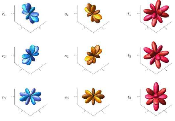
Different bases for the vector spacesH2d⊂V2dof harmonic polynomials are used in applications. A frequent choice in practice is the basis ofspherical harmonics[AH12] which are usually given as functions in spherical coordinates. In Section 5, we shall construct another basis for H2d that exhibits certain symmetries with respect to the group of signed permutations.
3. The Slice Method
Our aim is to determine a generating set of rational invariants for the linear action of the orthogonal group O3on the vector spacesV2d of even degree ternary forms. The group O3 is infinite and of dimension 3 as an algebraic group. We reduce the problem to the simpler question of determining rational invariants for the linear action of afinite group B3(contained in O3as a subgroup) on a subspace Λ2d ofV2d.
3.1. The Slice Lemma. We now introduce the general technique for the reduction mentioned above, called theslice method. For the formulation, we abstract from our specific setting: We consider a linear action of an algebraic group G on a finite-dimensionalR-vector spaceV, denoted
G×V →V, (g, v)7→gv.
In our particular case, we have G = O3 and V =V2d, and the action is defined in Section 2.1. We denote byR(V) the field of rational functions and by R(V)G the finitely generated subfield of rational invariants, as introduced already forV =V2d and G = O3.
The main technique for the announced reduction is known as theSlice Method[CTS07, Section 3.1], [Pop94].
It is based on the following definition.
Definition 3.1. Consider a linear group action of an algebraic group Gon a finite-dimensional R-vector spaceV. A subspaceΛ⊂V is called aslice for the group action, and the subgroup
B :={g∈G|gs∈Λ ∀s∈Λ} ⊂G is called its stabilizer, if the following two properties hold:
(i) For a general point v∈V there existsg∈Gsuch that gv∈Λ.
(ii) For a general points∈Λ the following holds: Ifg∈Gis such that gs∈Λ, theng∈B.
The Slice Lemma then states that rational invariants of the action of G onV are in one-to-one correspondence with rational invariants of the smaller group B⊂G on the slice Λ⊂V:
Theorem 3.2 (Slice Lemma). Let Λ be a slice of a linear action of an algebraic group G on a finite- dimensionalR-vector spaceV, and letBbe its stabilizer. Then there is a field isomorphism over Rbetween rational invariants
%:R(V)G−∼=→R(Λ)B, p7→p|Λ, which restricts a rational invariantp:V 99KRtop|Λ: Λ99KR.
This observation goes back to [Ses62], and we refer to [CTS07, Theorem 3.1] for a proof. Explicitly, the inverse to%:R(V)G−∼=→R(Λ)B is given by
%−1:R(Λ)B→R(V)G,
q7→ V 99KR, v7→q(gv), whereg∈G such thatgv∈Λ .
We will apply Theorem 3.2 for G = O3,V =V2d and a suitable choice for the slice Λ. The consequence of Theorem 3.2 for the construction of a generating set of rational invariants is the following.
Corollary 3.3. Let Λ be a slice of a linear action of an algebraic groupGon a finite-dimensionalR-vector space V, and let B be its stabilizer. If I = {p1, . . . , pm} is a generating set of rational invariants for the action ofBonΛ, thenJ:={%−1(p1), . . . , %−1(pm)}is a generating set of rational invariants for the action of GonV (where %is given as above).
Proof. Let p0 ∈ R(V)G. By assumption, %(p0) ∈ R(Λ)B can be written as a rational expression in the generators p1, . . . , pm. Since % is a field isomorphism, p0 = %−1(%(p0)) is the same rational expression in
%−1(p1), . . . , %−1(pm).
A corresponding statement for polynomial invariants requires much stronger hypotheses on the slice. In particular, even if the generating set forR(Λ)B consists ofpolynomial expressions p1, . . . , pm ∈R[Λ]B, the construction described above typically introduces denominators, so that %−1(p1), . . . , %−1(pm) ∈ R(V)G becomerational expressions.
3.2. A slice for V2d. We now describe a slice Λ2d ⊂V2d for the action of O3 onV2d for anyd≥1.
We recall from Section 1.1 the description of the action of O3 onV2: Elements of V2 are ternary quadratic forms and they can be identified with symmetric 3×3-matrices as in (1.3). If the associated symmetric matrix ofv∈V2isA, then for anyg∈O3⊂R3×3, the associated symmetric matrix ofgv∈V2is the matrix productgAgT.
Definition 3.4. Let Λ2⊂V2 denote the subspace of quadratic forms whose associated symmetric matrix is diagonal. Explicitly,
Λ2={λ1x2+λ2y2+λ3z2∈V2|λ1, λ2, λ3∈R}.
Ford≥2 we consider the Harmonic Decomposition ofV2dfrom Theorem 2.8 and defineΛ2d⊂V2d to be the subspace
Λ2d:=H2d⊕qH2d−2⊕ · · · ⊕qd−2H4⊕qd−1Λ2.
In other words, elements of the subspace Λ2d are thosev∈V2d that can be written as v=h2d+ qh2d−2+ q2h2d−4+. . .+ qd−2h4+ qd−1v0
with h2k ∈ H2k and v0 ∈Λ2 a quadratic form whose associated symmetric matrix is diagonal. The main observation is now the following:
Proposition 3.5. Letd≥1. The subspaceΛ2d⊂V2d is a slice for the action ofO3onV2dand its stabilizer is the group B3 ⊂O3 of signed permutation matrices. In particular, there is a one-to-one correspondence between rational invariants
%:R(V2d)O3−∼=→R(Λ2d)B3 given by the restriction of rational functions.