HAL Id: tel-00690743
https://tel.archives-ouvertes.fr/tel-00690743
Submitted on 24 Apr 2012
HAL is a multi-disciplinary open access archive for the deposit and dissemination of sci- entific research documents, whether they are pub- lished or not. The documents may come from teaching and research institutions in France or abroad, or from public or private research centers.
L’archive ouverte pluridisciplinaire HAL, est destinée au dépôt et à la diffusion de documents scientifiques de niveau recherche, publiés ou non, émanant des établissements d’enseignement et de recherche français ou étrangers, des laboratoires publics ou privés.
interface problems and its application to tumor growth model
Marco Cisternino
To cite this version:
Marco Cisternino. A parallel second order Cartesian method for elliptic interface problems and its application to tumor growth model. Modeling and Simulation. Université Sciences et Technologies - Bordeaux I; Politecnico di Torino, 2012. English. �NNT : �. �tel-00690743�
POLITECNICO DI TORINO
SCUOLA DI DOTTORATO Dottorato di Ricerca in Fluidodinamica
UNIVERSIT ´ E DE BORDEAUX 1
ECOLE DOCTORALE DE MATH´ ´ EMATIQUES ET INFORMATIQUE
Specialit´ e: Math´ ematiques Appliqu´ ees
Tesi di Dottorato - Th´ ese
A parallel second order Cartesian method for elliptic interface problems and its application to
tumor growth model
Marco Cisternino
Tutori - Directeurs:
prof. Angelo Iollo prof. Luca Zannetti
APRILE 2012
Abstract
This theses deals with a parallel Cartesian method to solve elliptic problems with complex interfaces and its application to elliptic irregular domain prob- lems in the framework of a tumor growth model. This method is based on a finite differences scheme and is second order accurate in the whole domain.
The originality of the method lies in the use of additional unknowns located on the interface, allowing to express the interface transmission conditions. The method is described and the details of its parallelization, performed with the PETSc library, are provided. Numerical validations of the method follow with comparisons to other related methods in literature. A numerical study of the parallelized method is also given. Then, the method is applied to solve elliptic irregular domain problems appearing in a three-dimensional continuous tumor growth model, the two-species Darcy model. The approach used in this ap- plication is based on the penalization of the interface transmission conditions, in order to impose homogeneous Neumann boundary conditions on the border of an irregular domain. The simulations of model are provided and they show the ability of the method to impose a good approximation of the considered boundary conditions.
Keywords: elliptic interface problem, Cartesian method, second order scheme, interface unknowns, parallel method, tumor growth, penalty method, elliptic irregular domain problem, homogeneous Neumann boundary conditions.
Abstract
Cette th`ese porte sur une m´ethode cart´esienne parall`ele pour r´esoudre des probl`emes elliptiques avec interfaces complexes et sur son application aux probl`e- mes elliptiques en domaine irr´egulier dans le cadre d’un mod`ele de croissance tumorale. La m´ethode est bas´ee sur un sch´ema aux diff´erences finies et sa pr´ecision est d’ordre deux sur tout le domaine. L’originalit´e de la m´ethode con- siste en l’utilisation d’inconnues additionnelles situ´ees sur l’interface et qui per- mettent d’exprimer les conditions de transmission `a l’interface. La m´ethode est d´ecrite et les d´etails sur la parall´elisation, r´ealis´ee avec la biblioth´eque PETSc, sont donn´es. La m´ethode est valid´ee et les r´esultats sont compar´es avec ceux d’autres m´ethodes du mˆeme type disponibles dans la litt´erature. Une ´etude num´erique de la m´ethode parall´elis´ee est fournie. La m´ethode est appliqu´ee aux probl`emes elliptiques dans un domaine irr´egulier apparaissant dans un mod`ele continue et tridimensionnel de croissance tumorale, le mod`ele `a deux esp`eces du type Darcy . L’approche utilis´ee dans cette application est bas´ee sur la p´enalisation des conditions de transmission `a l’interface, afin de imposer des conditions de Neumann homog`enes sur le bord d’un domaine irr´egulier. Les simulations du mod`ele sont fournies et montrent la capacit´e de la m´ethode `a imposer une bonne approximation de conditions au bord consid´er´ees.
Mots cl`es: probl`eme elliptique avec interface, m´ethode cart´esienne, sch´ema d’ordre deux, inconnues sur l’interface, m´ethode parall`ele, croissance tumorale, m´ethode de p´enalisation, probl`eme elliptique dans un domaine irr´egulier, con- ditions aux bords de Neumann homog`enes.
Abstract
Questa tesi introduce un metodo parallelo su griglia cartesiana per risolvere problemi ellittici con interfacce complesse e la sua applicazione ai problemi ellit- tici in dominio irregolare presenti in un modello di crescita tumorale. Il metodo
`e basato su uno schema alle differenze finite ed `e accurato al secondo ordine su tutto il dominio di calcolo. L’originalit`a del metodo consiste nell’introduzione di nuove incognite sull’interfaccia, le quali permettono di esprimere le condizioni di trasmissione sull’interfaccia stessa. Il metodo viene descritto e i dettagli della sua parallelizzazione, realizzata con la libreria PETSc, sono forniti. Il metodo
`e validato e i risultati sono confrontati con quelli di metodi dello stesso tipo trovati in letteratura. Uno studio numerico del metodo parallelizzato `e inoltre prodotto. Il metodo `e applicato ai problemi ellittici in dominio irregolare che compaiono in un modello continuo e tridimensionale di crescita tumorale, il modello a due specie di tipo Darcy. L’approccio utilizzato `e basato sulla pe- nalizzazione delle condizioni di trasmissione sull’interfaccia, al fine di imporre condizioni di Neumann omogenee sul bordo di un dominio irregolare. Le simu- lazioni del modello sono presentate e mostrano la capacit`a del metodo di imporre una buona approssimazione delle condizioni al bordo considerate.
Parole chiave: problema ellittico con interfaccia, metodo cartesiano, schema al secondo ordine, incognite sull’interfaccia, metodo parallelo, crescita tumorale, metodo di penalizzazione, problema ellittico in dominio irregolare, condizioni al bordo di Neumann omogenee.
Acknoledgements
I would like to thank all the people having followed me during the three Ph.D.
years. I do it without a special importance order because I don’t think I would be able to make a true ranking.
However, surely, the first place is for Angelo Iollo and Luca Zannetti. They give me the possibility of working with them, proposing me the subject of this thesis. Their experience and their advices have been a very important support to my work and to my scientific growth in general. My collaboration with them allows me to enter a new scientific domain and to enhance my formation from an international point of view. This work is surely the main effect of their trust in me.
A very special thanks goes to Lisl Weynans. Working with her has been an honor and a pleasure. We developed together the method, starting from an intial work of hers. We lived the development of the method together, having better and worse moments, discussing and improving. I want to thank her most of all for having encouraged me when the things seemed to get worse.
I want to show my gratitude to Olivier Saut for having introducing me to the domain of tumor growth modelling. The application of the method in the framework of his computational platform has been a strong boost for my work.
My sincere thanks to C´edric Galusinski and to Gabriella Puppo for having read and reported on the thesis. I really appreciate their advices and I am honored that my work has found their positive judgement.
I give thanks to all the MC2 ´equipe for the great welcome and the stimulating thirteen months spent working in it. Starting from its director, Thierry Colin, I want to thank Yannick, Jessica, Iraj, and all the others. Among them, a very special thanks to Michel Bergmann for having introducing me to Navier- Stokes simulation and for having made me taste the best Pessac-Leognan I’ve ever tasted. I will always remeber the wonderful ”holydays” in Maratea and in Porquerolles.
Thanks to Mathieu Specklin for a very nice and productive work period together. His help in developing the code was fundamental and his goodbye- party the best party I’ve been to in Bordeaux.
Another very special thanks goes to Damiano Lombardi. Sharing our works, ideas and passion for athletics was very interesting and enriching.
During the Bordeaux period I found very good friends: Franck, Adrien, Peng, C´edric, Michele, Johanna. Thanks a lot for your special help and all the funny moments together.
I want to give thanks to my office mate for the important and interesting english conversations about almost everything. He kept my english in training, correcting and improving me. It was very important, thanks Farhad.
A special thanks to Florian: his revision of the french (and not only) part of this manuscript has been very important.
special guys. The reasons are uncountable, scientifically and humanly. I met them in the Sala Alfa. Thanks a lot, Haysam and Federico, for the past and for the future.
This experience has given me a new dear friend, a football team mate and a collegue. His advices have been precious. I want to thank Edoardo.
A very special thanks to Miguel for all the things we did together before the beginning of this work and most of all for having urged me to start this adventure.
Thanks to all the Champisti: Davide, Mara, Roberta, Caterina, Sabino for your friendship and support.
Coming back home, even if just for a weekend, is always a special moment if you have wonderful old friends waiting for you. A huge ”thank you” to all my mates: Davide, Stette, Jalla, Umberto, Marcella, the whole Velvet Club, the Buenavista team, Stani, Davide.
For all the wholehearted support they have always given me and for a lot of other things I want to thank my family.
At the end, the most important thanks. No matter where I was or what I was doing, my thoughts were for her, always. She supported me in any case.
Staying away from home was hard for both me and her. I want to dedicate all my efforts to express her my infinite gratitude for having waited for me all the times and for all the love she gives me everyday. Thank you, Stefania.
Mobility Scholarships
This work has been conducted in the framework of a co-tutorship between the Politecnico di Torino and l’Universit´e Bordeaux 1. The mobility between this two institution has been possible thanks to the contributions of the following scholarships:
Bando UIF 2009
Contributi per il sostegno alla mobilit`a de dottorandi Universit`a Italo-Francese
Aide `a la mobilit´e `a l’international - Ann´ee 2011 Institut Polytechnique de Bordeaux
Programma Erasmus 2010/2011
Contents
1 Introduction 19
1.1 Motivation . . . 19
1.2 An overview of the work . . . 20
1.3 Structure of the work . . . 25
2 Introduzione (italiano) 27 2.1 Motivazione . . . 27
2.2 Una visione d’insieme del lavoro . . . 28
2.3 Struttura della tesi . . . 33
3 Introduction (fran¸cais) 35 3.1 Motivation . . . 35
3.2 Une vue d’enseble du travail . . . 36
3.3 Structure du travail . . . 41
4 A parallel second order Cartesian method for elliptic interface problems 43 4.1 Introduction to the method . . . 44
4.2 Convergence rate dependence on truncation error for the one- dimensional problem . . . 46
4.3 Description of the method for the two-dimensional problem . . . . 49
4.3.1 Interface description and classification of grid points . . . 49
4.3.2 Discrete elliptic operator for regular grid points . . . 50
4.3.3 Discrete elliptic operator near the interface . . . 50
4.3.4 Discrete flux transmission conditions . . . 51
4.3.5 Stabilization . . . 53
4.3.6 Caseα6= 0,β 6= 0 . . . 54
4.4 Three-dimensional extension by dimensional splitting . . . 55
4.5 Parallelization of the method . . . 58
4.5.1 Parallelization model and PETSc library . . . 58
4.5.2 Parallel implementation . . . 59
4.6 Numerical validation of the method . . . 63
4.6.1 Sequential validation of the method in two dimensions . . . . 63
4.6.2 Numerical study of the parallel method in two dimensions . . 76
4.6.3 A 3D simple case . . . 81
4.7 Conclusions about the method . . . 84 13
5 Application of the method to the tumor growth modelling 85
5.1 Introduction to the tumor growth modelling . . . 85
5.1.1 Brief notes on cancer biology . . . 85
5.1.2 Models . . . 87
5.2 The two-species Darcy model . . . 92
5.3 The numerical framework . . . 95
5.3.1 Domains . . . 96
5.3.2 The elliptic irregular domain problem . . . 98
5.3.3 Transport . . . 102
5.3.4 Discussion . . . 102
5.4 Simulations . . . 103
5.5 Conclusions about the application . . . 113
6 Future perspectives 115
List of Figures
1.1 Example of domain for elliptic interface problem . . . 20
1.2 Grid points classification . . . 21
1.3 2D Stencils . . . 22
1.4 3D Stencils . . . 22
2.1 Esempio di dominio per il problema ellittico con interfacce . . . 28
2.2 Classificazione dei punti griglia . . . 29
2.3 Stencils 2D . . . 30
2.4 Stencils 3D . . . 31
3.1 Exemple de domaine pour le probl`eme elliptique avec interface. . . 37
3.2 Classification des points du maillage . . . 37
3.3 Stencils 2D . . . 38
3.4 Stencils 3D . . . 39
4.1 Example of domain for elliptic interface problem . . . 44
4.2 Grid points classification . . . 50
4.3 Example of stencil for the discretization of the elliptic operator . . . . 51
4.4 Example of order two flux discretization at pointIi+1/2,j. . . 52
4.5 Example of order one flux discretization at pointIi+1/2,j. . . 52
4.6 Unstable flux discretization . . . 54
4.7 Stable flux discretization . . . 54
4.8 Example of 3D elliptic operator stencil near the interface . . . 56
4.9 Example of equation (4.3) stencil for the three-dimensional problem . 56 4.10 Example of stabilization for the three-dimensional problem . . . 58
4.11 Example of order one flux discretization for the three-dimensional problem . . . 58
4.12 Parallel matrix example. . . 60
4.13 Intersections arrangement . . . 61
4.14 Numerical solution for nx = ny = 120 for Problem 1 with k1 = 2 (u= 0 forr <1) . . . 65
4.15 Numerical error fornx=ny= 120 for Problem 1 withk1= 2 . . . 65
4.16 Numerical solution fornx =ny = 120 for Problem 1 withk1= 1000 (u= 0 forr <1) . . . 66
4.17 Numerical error fornx=ny= 120 for Problem 1 withk1= 1000 . . . 66
4.18 Numerical solution fornx=ny= 80 for Problem 2 . . . 67
4.19 Numerical error fornx=ny= 80 for Problem 2 . . . 68
4.20 Numerical solution fornx=ny = 80 for Problem 3 withk= 10 inside the interface . . . 69
4.21 Numerical error fornx =ny = 80 for Problem 3 with k = 10 inside the interface . . . 70
15
4.22 Numerical solution for nx = ny = 80 for Problem 3 with k = 1000
inside the interface . . . 70
4.23 Numerical error fornx=ny = 80 for Problem 3 withk= 1000 inside the interface . . . 71
4.24 Numerical solution fornx=ny= 80 for Problem 4 withb= 10 . . . . 73
4.25 Numerical error fornx=ny= 80 for Problem 4 withb= 10 . . . 73
4.26 Numerical solution fornx=ny= 80 for Problem 4 withb= 1000 . . . 74
4.27 Numerical error fornx=ny= 80 for Problem 4 withb= 1000 . . . . 74
4.28 Numerical solution fornx=ny= 80 for Problem 4 withb= 0.001 . . 75
4.29 Numerical error fornx=ny= 80 for Problem 4 withb= 0.001 . . . . 75
4.30 This figure shows how the calculation time scales with the number of processors. Crosses: experimental data in Table 4.11. Line: least square fit of the data. The experiments have been conducted on the machine Fourmi at PlaFRIM (see, [3]) . . . 77
4.31 Convergence test for Problem 5 withω= 5,r0= 0.5 andk− = 1000. Dashed line illustrates the slope of order two accuracy. Solid line is the slope of the linear regression. . . 78
4.32 Convergence test for Problem 5 withω= 12,r0= 0.4 andk−= 100. Dashed line illustrates the slope of order two accuracy. Solid line is the slope of the linear regression. . . 78
4.33 Numerical solution fornx=ny= 270 for Problem 5 forω= 5. . . 79
4.34 Numerical error fornx=ny= 270 for Problem 5 for ω= 5. . . 79
4.35 Numerical solution fornx=ny= 270 for Problem 5 forω= 12. . . 80
4.36 Numerical error fornx=ny= 270 for Problem 5 for ω= 12. . . 80
4.37 Numerical solution for the 3D test case. N x=Ny =Nz= 160,k1= 1 andk2= 1000 . . . 82
4.38 Numerical error for the 3D test case. N x=Ny =Nz = 160,k1 = 1 andk2= 1000 . . . 83
4.39 Scalability results on a 320×320×320 grid fork1= 1000 andk2= 1. 83 5.1 The cell cycle. From [8] . . . 86
5.2 CT-scans . . . 97
5.3 Segmented Lung . . . 97
5.4 Two-dimensional elliptic irregular domain problem test . . . 100
5.5 Hypoxia threshold . . . 103
5.6 Sphere. Initial condition . . . 104
5.7 Time evolution of the nodule shape. (Sphere case). . . 105
5.8 Time evolution of the nodule composition. (Sphere case). . . 106
5.9 Time evolution of oxygen concentration. (Sphere case). . . 107
5.10 Lung sides. . . 108
5.11 Initial geometrical setting . . . 108
5.12 Time evolution of the nodule shape. (Lung case, T=0-1.2). . . 109
5.13 Time evolution of the nodule shape. (Lung case, T=1.8-3.0). . . 110
5.14 Final time of the evolution of the nodule shape. (Lung case, T=5.0). . 111
5.15 Time evolution for oxygen concentration. (Lung case) . . . 112
5.16 Time evolution of the nodule composition. (Lung case). . . 113
List of Tables
4.1 Numericals results for Problem 1, fork1= 2 andk2= 1. . . 64 4.2 Numericals results for Problem 1, for k1 = 2 and k2 = 1, without
stabilization. . . 64 4.3 Numericals results for Problem 1, fork1= 1000 andk2= 1. . . 64 4.4 Numericals results for Problem 2 . . . 67 4.5 Numericals results for Problem 3, fork= 10 inside the interface . . . 69 4.6 Numericals results for Problem 3, fork= 1000 inside the interface . . 69 4.7 Numericals results inL∞norm for Problem 4,b= 10. . . 72 4.8 Numericals results inL∞norm for Problem 4,b= 1000. . . 72 4.9 Numericals results inL∞norm for Problem 4,b= 0.001. . . 72 4.10 Parallel numericals results for Problem 1, fork1= 1000 andk2= 1. . 76 4.11 Scalability results on a 3500×3500 grid for Problem 1. . . 76 4.12 Error convergence results for the three-dimensional test case withk1=
1000 andk2= 1. . . 81 4.13 Error convergence results for the three-dimensional test case withk1=
1 andk2= 1000. . . 82 5.1 Normal derivatives of the solution on∂Ω, varyingAand ˜k. . . 99
17
Chapter 1
Introduction
1.1 Motivation
Elliptic problems with discontinuous coefficients and sources are often encoun- tered in fluid dynamics, heat transfer, solid mechanics, electrodynamics, mate- rial science and biological modelling.
These physical problems have solutions consisting of several components sepa- rated by interfaces and for that reason they are often referred as elliptic interface problems. Such interfaces can be still or dynamically moving physical bound- aries, material interfaces, phase boundaries, etcetera.
A lot of efforts have been made dealing with these problems, using several differ- ent approaches and discretization techniques: finite elements methods on adap- tive grids, body-fitted finite difference and finite volume methods and Cartesian grid methods. The present work deals with the latter of these methods by combining it with finite difference schemes, the introduction of new auxiliary unknowns and a dimension-splitting approach.
Many other methods have been designed for solving elliptic interface problems on structured grids. In this work the aim is focused on simplicity of interface treatment, in order to exploit all the Cartesian grid advantages in guaranteeing an easy parallelization.
The high topology complexity of the interface and the need for solving an elliptic interface problem at each time step of a time integration method require that efficiency the parallel computing can give. On the other hand, the literature in elliptic interface problem area lacks in parallel methods which guarantee second order error convergence rate and sharp solutions. This motivated the present study, leading to the development of a parallel second order method for elliptic interface problems which gives accurate sharp solutions across the interface and is easy to be implemented by the use of already existing tools.
The widespread presence of the elliptic interface problems in many scientific do- mains, we mentioned at the beginning of this section, ensures several different application frameworks. Among them, the present method will get involved in modelling interface phenomena such as free surface dynamics, fluid-structure interaction or electric potential in biological cells. In the present work the ap- plication of the method to the elliptic irregular domain problem, close related to the elliptic interface problem, is provided.
Embedding an irregular domain in a regular one and considering boundary con- ditions as interface jump conditions the present method is exploited in a penalty method spirit to impose homogeneous Neumann conditions on a complex lung
19
surface, in order to solve pressure and nutrients equations in the framework of a tumor growth model. The lack in second order error convergence rate, up to the irregular lung boundary, of the methods previously employed in this model motivated this application.
1.2 An overview of the work
In this section an overview of the entire work is given. Without details, the main idea of the method and its parallelization are provided and we also touch on tumor growth model, showing details, results and simulations later on.
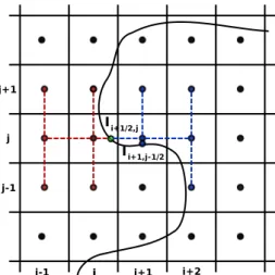
The aim of this work is to solve the problem, known as elliptic interface problem, described by the following system of partial differential equations
∇ ·(k∇u) = f on Ω = Ω1∪Ω2 (1.1)
JuK = α on Σ (1.2)
Jk∂u
∂nK = β on Σ (1.3)
with an order two accuracy on Cartesian grids, using finite differences schemes.
J·Kmeans·1− ·2. Ω is the whole computational domain and it is the set union of two sub-domains, Ω1 and Ω2, sharing a co-dimension 1 set, Σ, a complex interface. Opportune boundary conditions on ∂Ω, the Ω boundary, complete the system. Figure 1.1 shows an example of this kind of domain.
1
2
δ
Ω Ω
Ω
Ω Σ
Figure 1.1: Geometry considered: two sub-domains Ω1 and Ω2 separated by a complex interface Σ
In this problemk, the diffusion coefficient,f, the source,u, the solution and k∂u∂n, the co-normal derivative of the solution could have strong discontinuities across the interface.
Starting from an analysis of the convergence error, in terms of the truncation error, applied to the Laplacian operator in a ghost-point methods spirit, we deduce the needs for order two accuracy:
1.2. OVERVIEW 21
• a discretization of the Laplacian operator near the interface with a trun- cation error of order one,
• a discretization of the transmission conditions (1.2) and (1.3) at the inter- face with a truncation error of order two.
Therefore, we distinguish grid points between regular grid points, far more than a grid step from the interface, and interface grid points, close to the in- terface less than a grid step (Figure 1.2 gives an example). On the former we discretize the Laplacian operator using standard centred second order finite dif- ferences scheme. As far as the latter is concerned, in order to satisfy the order two accuracy requirements, we decide to introduce new unknowns, i.e. the val- ues of the solution at the intersections of the interface with the grid axes (see Figure 1.2).
j j+1
j-1
i
i-1 i+1 i+2
Figure 1.2: Grid points classification: regular grid points are in full black, interface grid points are in red-black and intersection points are in green-black.
Straight lines mark cells off.
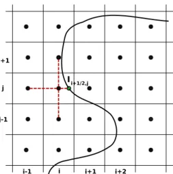
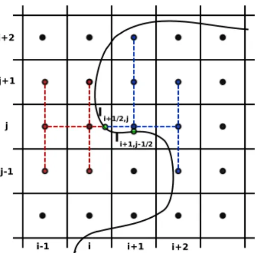
All these elements allow us to discretize on a Cartesian grid the whole system of equations (1.1 - 1.3). A sketch of the discretization stencils used near the in- terface for the Laplacian operator and at the interface for the co-normal solution derivative jump is given in Figure 1.3. Solution jump condition is embedded in equations (1.1) and (1.3) discretization as a contribution to the right-hand side.
Clearly, considering the nature of the approximation near the interface, we need information about the interface position and normals. Furthermore, the new variables need to be numbered, in order to assembly the linear system.
For the sake of parallelism, the better way to keep this information efficiently is to use a level set function for all the geometrical features of the interface and to store intersections numbering and position in a grid-based parallel data structure.
Two remarks are necessary. Firstly, it is not always possible to discretize the transmission condition (1.3) with a second order truncation error; as the matter of fact doing it needs at least two aligned points on the same side of the interface; when it is not possible a first order truncation error discretization is used. Secondly, the tangential derivative jump condition at the interface can
j j+1
j-1
i-1 i i+1 i+2
I i+1/2,j
(a) Laplacian operator stencil
j j+1
j-1
i-1 i i+1 i+2
I i+1/2,j
(b) Equation 1.3 stencil
Figure 1.3: 2D stencils used near the interface.
be deduced from the solution jump condition and used to reduce the number of points involved in the stencil in Figure 1.3b. Some tests have been made and no significant improvements in solution accuracy or in computational performance have been observed.
Preliminary tests, using the scheme we have just touched on here, show insta- bilities in error convergence rate. For this reason we decide to slightly modify the condition (1.3) stencil, preventing the presence of too close intersections.
This gives far smoother error convergence curves.
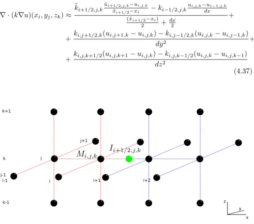
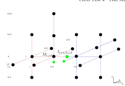
The extension of the method to the three-dimensional problem is straightfor- ward, thanks to the dimensional splitting approach. An example of the stencils involved in this problem is in Figure 1.4.
(a) Laplacian operator stencil
(b) Equation 1.3 stencil
Figure 1.4: 3D stencils used near the interface. Green balls for intersections.
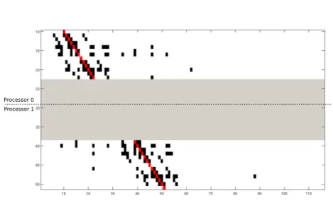
As far as the parallelization of the method is concerned, the use of the level set function and storing out-of-grid points information (the intersection points) as properties of the grid points allow an easy application of the local memory paradigm for parallelism, by using the PETSc library. The domain decomposi- tion is accomplished just paying attention to the intersections numbering. This arrangement is performed trying to reduce the number of message passing com-
1.2. OVERVIEW 23 munications and keeping the processors load disproportion as low as we can.
Finally the parallel code is written using already existing tool, almost without explicitly taking care of the communications.
The numerical validation of the method is carried out providing convergence results for five different two-dimensional test cases and for a preliminary easy three-dimensional test case, using the parallel and the sequential implementa- tions. Error convergence rates show a satisfying second order accuracy even on complex interfaces and the comparisons with other methods in literature prove a competitive absolute error.
The scalability performances of the parallel implementation are tested for both the two-dimensional and the three-dimensional problem, considering the simplest test cases. The results show a good scaling between the computational time and the number of processors, not too far from the perfect parallelism.
Our method is consequently applied to solve the elliptic irregular domain problems appearing in a three-dimensional continuous tumor growth model, specifically the two-species Darcy model.
The continuous model, by means of PDEs, can take into account the space evolution, providing information about the shape and the location of the tumor during its evolution. Among these models the most complex ones are usually not suitable for clinic applications, because of their huge number of free parameters to be determined.
The present application has to be considered in the framework of free pa- rameters identification problem. In this framework inverse problems have to be solved and too many free parameters can make this task computationally im- possible. The two-species Darcy model is able to give a reasonable description of the phenomena, surely not considering certain biological mechanisms, but because of its reduced number of free parameters relative to more sophisticated models, it is able to offer an affordable identification problem.
The model describes a three phases saturated flow in a porous isotropic non- uniform medium. P, Q and S are, respectively, the number of proliferating (dividing, responsible for the tumor growth), quiescent and healthy cells per unit volume and the equations for them read:
∂P
∂t +∇ ·(~vP) = (2γ−1)P+γQ (1.4)
∂Q
∂t +∇ ·(~vQ) = (γ−1)P−γQ (1.5)
∂S
∂t +∇ ·(~vS) = 0 (1.6)
where the velocity~v accounts for the tissue deformation and γ, a scalar func- tion of the nutrients, determines if the tumor cells proliferate or die (becoming quiescent). Passive motion is assumed. The saturated flow hypothesis is used, P+Q+S= 1, which implies
∇ ·~v=γP (1.7)
and the mechanical clusure of the system is given by a Darcy law for the velocity
~v=−k(P, Q)∇Π (1.8)
where Π is a scalar function playing the role of a pressure (or potential) andk is the permeability field given by
k=k1+ (k2−k1)(P+Q) (1.9)
being k1 the constant permeability of the healthy tissue and k2 the constant permeability of the tumor tissue.
The nutrients (specifically, the oxygen) are governed by a diffusion-reaction equation:
∂tC− ∇ ·(D(P, Q)∇C) = 0.1(Cmax−C)S−αP C−0.01αQC (1.10) whereCis the density of nutrients,Cmax= 1 andαis the nutrients consumption rate for the proliferating cells.
D=Dmax−K(P+Q) (1.11)
is the diffusivity expressed by a phenomenological law reflecting the different diffusion of the oxygen in healthy and tumor tissues.
Theγfunction expresses the transition between the proliferating and quies- cent state and it is the regularization of the unit step
γ=1 + tanh(R(C−Chyp))
2 (1.12)
whereR is a coefficient andChypis the hypoxia threshold.
The domain, Ω, is generally a complex domain with an irregular bound- ary. No mass can leave this domain and for this reason homogeneous Neumann boundary conditions are imposed for both the oxygen and the pressure equa- tions. But the Neumann problem for the pressure has to be well posed, then a modification of the velocity divergence is needed: it has to be a zero average scalar quantity and so
∇ ·~v=γ(C)− R
ΩγP dΩ R
Ω1−P−Q dΩ(1−P−Q). (1.13) This correction means a compression of the healthy tissue caused by the tumor growth and consequently the equation (1.6) can no longer hold.
Our method is introduced to solve the equation for the pressure (1.8) and for the nutrients (1.10) in an irregular domain. The original domain Ω is embedded in a larger regular one Ω′. The original boundary conditions are considered as transmission conditions at the interface separating Ω and its relative component in Ω′, introducing new permeability and diffusivity
k′ =
(k, in Ω
kout, in Ω′\Ω (1.14)
D′ =
(D, in Ω
Dout, in Ω′\Ω (1.15)
In the spirit of a penalty method we impose approximated homogeneous Neu- mann boundary conditions for pressure and oxygen at the boundary of Ω, choos- ing very small values forkout andDout.
1.3. STRUCTURE 25 We perform two simulations of the model with different geometries and initial conditions. The aim is to show the importance of three-dimensional modelling in tumor growth and the role played by the boundary of Ω in the evolution of a tumor nodule shape. The interfaces (boundaries of Ω) chosen are a sphere and a lung. The latter is obtained by segmentation of medical images (CT- scans). The results provide, on a quality level, a good behaviour of the method in imposing the homogeneous Neumann boundary conditions on the border of Ω and a reasonable evolution of the nodule shape and composition.
Error convergence studies with more complex three-dimensional interfaces as well as quantitative results and comparisons with realistic cases in tumor growth simulation are needed to corroborate what is shown in the present work.
Managing more than one interface, then more than two different sub-domains is an important improvement not only for the method itself, but for the tumor growth model too. This can introduce the possibility of considering a struc- tured, and therefore more realistic, original domain. These are the main future perspectives of this work.
1.3 Structure of the work
Inchapter 4the parallel second order method for elliptic interface problems is introduced.
Insection 4.1an overview about the existing and the present method is given.
The successivesection 4.2 provides the genesis of the main idea, analysing the convergence error for the one-dimensional problem.
Insection 4.3the detailed description of the method is illustrated for the two- dimensional problem.
Afterwards, insection 4.4, the dimensional splitting is used to give some details about the method for the three-dimensional problem.
The parallel implementation is introduced insection 4.5with highlights on the model adopted, on the tools used and on the arrangement of the linear system.
Thesection 4.6 provides the numerical validation of the method, showing the error convergence rate results for a good range of two-dimensional test cases, using both sequential and parallel implementations. A simple three-dimensional test case and the scalability performances of the parallel implementation are also discussed in this section.
The chapter ends with the conclusions about the method in section 4.7.
In chapter 5 the method is applied to solve the elliptic irregular domain problem in the framework of a tumor growth model.
Insection 5.1 a brief introduction to tumor growth modelling is given and the chosen model is illustrated in section5.2.
Afterwards, insection 5.3 the whole numerical application framework is intro- duced. We show how our method can be used to solve the elliptic irregular domain problem and some notes about medical imagery and segmentation tools are provided in order to show how the geometries involved have been obtained.
Finally, insection 5.4the results of the simulations are shown and discussed.
Conclusions about the application conclude the chapter, insection 5.5.
Perspectives and future intentions about the method itself, the tumor growth model and the alternative applications of the method are discussed inchapter 6.
Chapter 2
Introduzione (italiano)
2.1 Motivazione
I probelmi ellittici con sorgenti e coefficienti discontinui sono comuni nella flu- idodinamica, nella trasmissione del calore, in meccanica dei solidi, in elettrodi- namica, nelle scienze dei materiali e nella modellistica biologica.
Le soluzioni di questi problemi fisici consistono in diverse componenti separate da interfacce e per questo motivi sono spesso conosciuti come problemi ellittici con interfacce. Tali interfacce possono essere contorni fisici stazionari o mobili, interfacce materiali, contorni di fase, eccetera.
Molti sforzi sono stati compiuti trattando questi problemi, facendo uso di molti e differenti approcci e tecniche di discretizzazione: metodi agli elementi finiti su griglie adattative, metodi ai volumi finiti e alle differenze finite su griglie adattate e metodi su griglia cartesiana. Questo lavoro tratta l’ultimo di questi metodi combinandolo con gli schemi alle differenze finite, con l’introduzione di nuove incognite ausiliarie e con un approccio dimensione-per-dimensione.
Molti altri metodi sono stati sviluppati per risolvere i problemi ellitici con in- terfacce su griglie strutturate. In questo lavoro vogliamo porre l’accento sulla semplicit`a di trattamento dell’interfaccia, al fine di sfruttare tutti i vantaggi di una griglia cartesiana garantendo una facile parallellizzazione.
L’elevata complessit`a topologica dell’interfaccia e la necessit`a di risolvere un problema ellittico con interfaccia ad ogni passo temporale di un metodo di inte- grazione in tempo richiedono un livello di efficienze che il calcolo parallelo pu`o fornire. D’altro canto, la letteratura relativa al problema ellitico con interfaccia
`e priva di metodi paralleli che garantiscano un tasso di convergenza dell’errore del secondo ordine e soluzioni nette all’interfaccia. Ci`o ha motivato il presente studio, portandoci allo sviluppo di un metodo al secondo ordine parallelo per problemi ellittici con interfacce capace di fornire soluzioni nette e discontinue attraverso l’interfaccia e facile da implementare grazie all’uso di strumenti es- istenti.
La diffusa presenza dei problemi ellittici con interfacce in molti campi scientifici, menzionata all’inizio di questa sezione, assicura numerosi e differenti contesti applicativi. Tra questi, il metodo attuale verr`a impiegato nella modellizzazione di fenomeni d’interfaccia quali la dinamica di un’interfaccia libera, l’interazione fluido-struttura o lo studio del potenziale elettrico in cellule biologiche. In questo lavoro l’applicazione del metodo al problema ellittico in dominio irregolare, stret- tamente connesso al problema ellittico con interfaccia, `e fornita.
Inserendo un dominio irregolare in uno regolare e considerando le condizioni 27
al bordo come condizioni di salto, il presente metodo `e sfruttato nello spirito di un metodo di penalizzazione per imporre condizioni di Neumann omogenee sulla superficie di un polmone complesso, al fine di risolvere le equazioni per la pressione e per i nutrienti nel contesto di un modello di crescita tumorale.
La mancanza di un tasso di convergenza al secondo ordine dell’errore, in re- gioni prossime al contorno del polmone, nei metodi precedentemente impiegati in questo modello ha motivato questa applicazione.
2.2 Una visione d’insieme del lavoro
In questa sezione viene fornita una panoramica dell’intero lavoro. Senza dettagli, proponiamo l’idea principale del metodo e la sua parallelizzazion e accenniamo al modello di crescita tumorale, mostrando dettagli, risultati e simulazioni pi´u avanti.
Lo scopo di questo lavoro `e risolvere il problema, noto come problema ellittico con interfacca, descritto dal seguente sistema di equazioni alle derivate parziali
∇ ·(k∇u) = f on Ω = Ω1∪Ω2 (2.1)
JuK = α on Σ (2.2)
Jk∂u
∂nK = β on Σ (2.3)
al secondo ordine di accuratezza su griglie cartesiane, utilizzando schemi alle differenze finite. J·K sta per ·1− ·2. Ω `e l’intero dominio computazionale ed `e l’unione di due sottodomini, Ω1 e Ω2, che condividono un insieme di codimen- sione 1, Σ, un interfaccia complessa. Opportune condizioni al bordo su ∂Ω, il bordo di Ω, completano il sistema. Figura 2.1 mostra un esempio di questo tipo di dominio.
1
2
δ
Ω Ω
Ω
Ω Σ
Figure 2.1: Geometria considerata: due sottodomini Ω1 e Ω2 separati da un’interfaccia complessa Σ
In questo problema, k, il coefficiente di diffusione, f, la sorgente, u, la soluzione e k∂u∂n, la derivata conormale della soluzione potrebbero avere forti discontinuit`a attraverso l’interfaccia.
2.2. VISIONE D’INSIEME 29 Partendo dall’analisi dell’errore di convergenza, in termini dell’errore di tron- camento, applicata all’operatore laplaciano nello spirito dei metodi ghost-point, deduciamo quali richieste dobbiamo soddisfare per ottenere un’accuratezza al secondo ordine:
• una discretizzazione nei pressi dell’interfaccia dell’operatore di Laplace con un errore di troncamento di ordine uno.
• una discretizzazione delle condizioni di trasmissione (2.2) e (2.3) all’interfaccia con un errore di troncamento di ordine due.
Perci`o, distinguiamo i punti della griglia in punti regolari, lontani pi´u di un passo griglia dall’interfaccia, e in punti di interfaccia, a meno di un passo griglia dall’interfaccia (Figura 2.2 d`a un esempio). Sui primi discretiziamo l’operatore di Laplace usando lo schema alle differenze finite centrato standard al secondo ordine. Per quanto riguarda i secondi, al fine di soddisfare le richieste relative all’accuratezza di ordine due, decidiamo di introdurre nuove incognite, ovvero i valori della soluzione nelle intersezioni dell’interfaccia con gli assi della griglia (see Figure 2.2).
j j+1
j-1
i
i-1 i+1 i+2
Figure 2.2: Classificazione dei punti griglia: i punti griglia regolari in nero pieno, punti griglia d’interfaccia sono in rosso-nero e i punti d’intersezione in verde-nero. Linee continue contornano le celle.
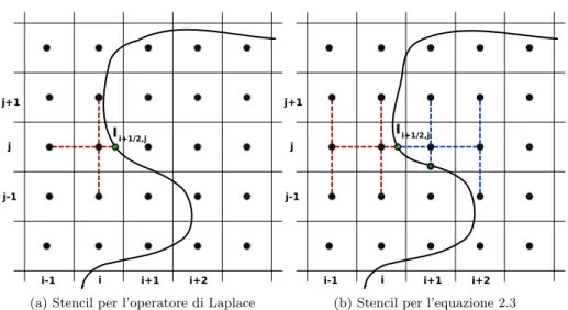
Gli elementi sin qui introdotti ci permettono di discretizzare l’intero sis- tema di equazioni (2.1 - 2.3) su una griglia cartesiana. Una rappresentazione grafica degli stencils di discretizzazione utlizzati nei punti vicini all’interfaccia per l’operatore di Laplace e sull’interfaccia per il salto della derivata conormale della soluzione `e proposta in Figura 2.3. La condizione di salto per la soluzione
`e inserita nella discretizzazione delle equazioni (2.1) and (2.3) come contributo al termine noto.
E evidente che, considerando la natura dell’approssimazione, abbiamo bisogno` di informazione sulla posizione dell’interfaccia e sulle normali all’interfaccia stessa. Inoltre, le nuove variabili devono essere numerate per poter consistente- mente assemblare il sistema lineare. Per una buona implementazione parallela, il modo migliore di conservare efficientemente tali informazione `e di utilizzare
j j+1
j-1
i-1 i i+1 i+2
I i+1/2,j
(a) Stencil per l’operatore di Laplace j j+1
j-1
i-1 i i+1 i+2
I i+1/2,j
(b) Stencil per l’equazione 2.3
Figure 2.3: Stencils 2D impiegati nei pressi dell’interfaccia.
una funzione level set per tutte le caratteristiche geometriche dell’interfaccia e di immagazzinare la numerazione e la posizione delle intersazioni in una struttura parallela basata sulla griglia.
A questo punto sono necessarie due osservazioni. In primo luogo, non `e sempre possibile discretizzare la condizione di trasmissione (2.3) con un errore di troncamento al secondo ordine; infatti per far ci`o abbiamo bisogno di al- meno due punti allineati sullo stesso lato dell’interfaccia; quando questo non `e possibile una discretizzazione con errore di troncamento al primo ordine viene utilizzata. In secondo luogo, la condizione di salto all’interfaccia per la derivata tangenziale della soluzione pu`o essere dedotta dalla condizione di salto della soluzione e utilizzata per ridurre il numero di punti coinvolti nello stencil in Figura 2.3b. Alcuni tests hanno dimostrato che nessun miglioramento signi- ficativo nell’accuratezza della soluzione o nella prestazione computazionale pu`o essere apprezzato.
Tests preliminari, utilizzando lo schema sin qui accennato, mostrano in- stabilit`a nel tasso di convergenza dell’errore. Per questo motivo decidiamo di modificare leggermente la discretizzazione della condizione (2.3), impedendo la presenza di intersezioni troppo vicine nello stesso stencil. Ci`o fornisce curve di convergenza dell’errore molto pi´u lisce.
L’estensione del metodo al problema tridimensionale `e semplice considerando ogni direzione in maniera indipendente. Un esempio degli stencils coinvolti in tale problema `e dato in Figura 2.4.
Per quanto riguarda la parallelizzazione del metodo, l’uso della funzione level set e l’immagazzinare l’informazione dei punti fuori griglia (i punti d’intersezione) come propriet`a dei punti della griglia permettono una facile applicazione del paradigma di programmazione parallela a memoria locale, attraverso l’uso della libreria PETSc. La decomposizione di dominio `e ottenuta semplicemente facendo attenzione alla numerazione delle intersezioni. Tale numerazione `e compiuta cer- cando di ridurre il numero di comunicazioni message passing and di tenere il divario tra i carichi dei processori il pi´u basso possibile. Infine il codice parallelo
2.2. VISIONE D’INSIEME 31
(a) Stencil per l’operatore di Laplace
(b) Stencil per l’equazione 2.3
Figure 2.4: Stencils 3D impiegati nei pressi dell’interfaccia. Le sfere verdi rap- presentano le intersazioni.
`e scritto utilizzando strumenti gi`a esistenti, quasi senza occuparsi esplicitamente delle comunicazioni.
La validazione numerica del metodo `e realizzata fornendo risultati di conver- genza per cinque diversi casi bidimensionali a per un semplice e preliminare caso tridimensionale, utilizzando le implementazioni sequanziale e parallela. I tassi di convergenza dell’errore mostrano una soddisfacente accuratezza al secondo ordine anche su interfacce complesse e i confronti con altri metodi in letteratura provano un errore assoluto competitivo.
Le prestazioni di scalabilit`a dell’implementazione parallela sono testate sia per il problema bidimensionale che per quello tridimensionale, considerando i casi pi´u semplici. I risultati mostrano un buon comportamento del tempo di calcolo in funzione del numero di processori, non troppo lontano dal parallelismo perfetto.
Il nostro metodo `e conseguentemente applicato per risolvere i problemi ellit- tici in dominio irregolare che compaiono nel modello continuo e tridimensionale di crescita tumorale, specificatamente il modello a due specie di Darcy.
Il modello continuo, per mezzo di EDP, `e in grado di considerare l’evoluzione spaziale, fornendo informazioni sulla forma e la localizzazione del tumore du- rante il suo sviluppo. Tra questi modelli i pi´u complessi non sono solitamente adatti ad applicazioni cliniche, a causa dell’elevato numero di parametri liberi da determinare.
La presente applicazione deve essere considerata nel contesto del problema di identificazione dei parametri liberi di un modello. In questo contesto `e necessario risolvere dei problemi inversi e troppi parametri liberi possono rendere questo obiettivo computazionalmente impossibile. Il modello a due specie di Darcy pu`o dare una ragionevole descrizione del fenomeno, pur non considerando alcuni meccanismi biologici, ma a causa del suo ridotto numero di parametri liberi rispetto a modelli pi´u sofisticati, `e in grado di offrire un accessibile problema di identificazione.
Il modello descrive il flusso saturo di tre fasi in un mezzo poroso non uniforme e isotropo.
P, Q eS sono, rispettivamente, il numero di cellule proliferanti (capaci di dividersi e responsabili della crescita tumorale), quiescenti e sane per unit`a di
volume e le equazioni che le governano sono:
∂P
∂t +∇ ·(~vP) = (2γ−1)P+γQ (2.4)
∂Q
∂t +∇ ·(~vQ) = (γ−1)P−γQ (2.5)
∂S
∂t +∇ ·(~vS) = 0 (2.6)
dove la velocit`a ~v rende conto della deformazione tissutale e γ, una funzione scalare dei nutrienti, determina se le cellule tumorali proliferano o muoiono (diventando quiescenti). Si assume moto passivo. L’ipotesi di flusso saturo `e introdotta,P+Q+S= 1, la quale implica
∇ ·~v=γP (2.7)
e la chiusura meccanica del sistema `e data da una legge di Darcy per la velocit`a
~v=−k(P, Q)∇Π (2.8)
dove Π `e una funzione scalare che gioca il ruolo di pressione (o potenziale) ek
´e il campo di permeabilit`a dato da
k=k1+ (k2−k1)(P+Q) (2.9)
essendok1la permeabilit`a costante del tessuto sano ek2la permeabilit`a costante del tessuto tumorale.
I nutrienti (specificatamente, l’ossigeno) sono governati da un’equazione di reazione-diffusione:
∂tC− ∇ ·(D(P, Q)∇C) = 0.1(Cmax−C)S−αP C−0.01αQC (2.10) dove C`e la densit`a di nutrienti, Cmax= 1α`e il tasso di consumo di nutrienti ad opera delle cellule proliferanti.
D=Dmax−K(P+Q) (2.11)
`e la diffusivit`a espressa da una legge fenomenologica che rispecchia le differenti diffusioni dell’ossigeno nei tessuti sano e tumorale.
La funzione γ regola la transizione tra gli stati proliferante e quiescente ed
`e la regolarizzazione del gradino unitario
γ=1 + tanh(R(C−Chyp))
2 (2.12)
dove R`e un coefficiente eChyp`e la soglia di iposs´ıa.
Il dominio, Ω, `e generalmente un dominio complesso con un contorno irre- golare. La massa interna al dominio non pu`o uscire dal dominio stesso, quindi condizioni al contorno di Neumann omogenee sono imposte sia per l’ossigeno che per la pressione. Ma il problema di Neumann per la pressione deve essere ben posto, quindi `e necessario modificare la divergenza della velocit`a: deve essere una quantit`a scalare a media nulla nel dominio e dunque
∇ ·~v=γ(C)− R
ΩγP dΩ R
Ω1−P−Q dΩ(1−P−Q). (2.13)
2.3. STRUTTURA 33 Tale correzione implica una compressione del tessuto sano causata dalla crescita del tumore e conseguentemente l’equazione (2.6) non `e pi´u valida.
Il nostro metodo `e introdotto per risolvere le equazioni per la pressione (2.8) e per i nutrienti (2.10) in un dominio irregolare. Il dominio originale Ω viene quindi inserito in uno pi´u grande e regolare Ω′. Le condizioni al contorno origi- nali sono considerate come condizioni di trasmissione all’interfaccia che separa Ω e il suo complemento relativo in Ω′, introducendo nuove permeabilit`a e diffu- sivit`a.
k′=
(k, in Ω
kout, in Ω′\Ω (2.14)
D′=
(D, in Ω
Dout, in Ω′\Ω (2.15)
Utilizzando un metodo di penalizzazione, imponiamo un’approssimazione delle condizioni al contorno di Neumann omogenee per la pressione e per l’ossigne al bordo di Ω, scegliendo valori perkout eDout molto piccoli.
Realizziamo due simulazioni del modello con differenti geometrie e condizioni iniziali. Lo scopo ´e di mostrare l’importanza della modellizzazione tridimension- ale della crescita tumorale e il ruolo giocato dal contorno di Ω nell’evoluzione della forma del nodulo tumorale. Le interfacce (contorni di Ω) scelte sono una sfera e un polmone. Quest’ultimo `e ottenuto per segmentazione di immagini medicali (scansioni di CT). I risultati forniscono, ad un livello qualitativo, un buon comportamento nell’imporre le condizioni al contorno di Neumann omo- genee da parte del metodo e una ragionevole evoluzione della forma e della composizione del nodulo.
Studi di convergenza dell’errore con interfacce tridimensionali pi´u complesse cos´ı come risultati quantitativi e confronti con casi realistici per quanto riguarda la crescita tumorale sono necessari per corroborare ci`o che `e mostato nel pre- sente lavoro. These are the main future perspectives of this work. Gestire la presenza di pi´u interfacce, quindi pi´u di due sottodomini `e un miglioramento importante non solo per il metodo in s´e ma anche per il modello di crescita tumorale. Ci`o infatti introdurrebbe la possibilit`a di considerare un dominio originale strutturato e quindi pi´u realistico. Queste sono le prospettive future principali di questo lavoro.
2.3 Struttura della tesi
Nelcapitolo 4il metodo parallelo al secondo ordine per problemi ellittici con interfaccia `e introdotto.
Nellasezione 4.1 una panoramica dei metodi esistenti e del presente metodo `e data.
La successiva sezione 4.2 fornisce la genesi dell’idea principale, analizzando l’errore di convergenza per il problema unidimensionale.
Nella sezione 4.3 la descrizione dettagliata del metodo viene illustrata per il problema bidimensionale.
Successivamente, nellasezione 4.4, lo splitting dimensionale `e usato per fornire qualche dettaglio circa il metodo per i problemi tridimensionali.
L’implementazione parallela `e introdotta nellasection 4.5sottolineando il mod- ello introdotto, gli strumenti di programmazione impiegati e l’organizzazione del sistema lineare.
Laseezione 4.6fornisce la validazione numerica del metodo, mostrando i risultati sui tassi di convergenza dell’errore per un buon intervallo di casi bidimensonali, utilizzando sia l’implementazione parallela che quella sequanziale. Un semplice caso tridimensionale e le prestazioni di scalabilit`a dell implementazione paralle sono pure discussi in questa sezione.
Il capitolo termina con le conclusione circa il metodo in sezione 4.7.
Nel capitolo 5 il metodo `e applicato per risolvere il problema ellittico in dominio irregolare nel contesto di un modello di crescita tumorale
Nella sezionesection 5.1una breve introduzione alla modellizzazione di crescita tumorale `e data e il modello scelto `e illustrato nella sezione5.2.
Successivamente, nella sezione 5.3 l’intero contesto numerico dell’applicazione
`e introdotto. Mostriamo come il nostro metodo pu`o essere usato per risolvere il problema ellittico in dominio irregolare e qualche cenno alla dignostica per immagini e agli strumenti di segmentazione `e fornito per mostrare come le ge- ometrie coinvolte sono state ottenute.
In fine, nellasezione 5.4i risultati delle simulazioni sono mostrati e discussi.
Le conclusioni circa l’applicazione concludono il capitolo insezione 5.5.
Le propsettive e le intenzioni future sul metodo, sul modello di crescita tumorale e sulle applicazioni alternative del metodo sono discusse nelcapitolo 6.
Chapter 3
Introduction (fran¸cais)
3.1 Motivation
Les probl`emes elliptiques avec coefficients et sources discontinues sont sou- vent rencontr´es dans la m´ecanique des fluides, la transmission de la chaleur, la m´ecanique des solides, l’´electrodynamique, la science des mat´eriels et la mod´elisation biologique.
Les solutions de ces probl`emes physiques sont faites de plusieurs composantes s´epar´ees par des interfaces et pour cette raison ils sont souvent appel´es probl`emes elliptiques avec interfaces. Telles interfaces peuvent ˆetre contours physiques sta- tionnaires ou mobiles, interfaces mat´erielles, contours de phase, et cetera.
Beaucoup d’efforts ont ´et´e faits pour r´egler ces probl`emes en utilisant plusieurs approches et techniques de discr´etisation : m´ethodes `a ´el´ements finis sur mail- lages adaptatifs, m´ethodes `a diff´erences finies et volumes finis sur maillages adapt´es au corps et m´ethodes sur maillages cart´esiens.
Ce travail concerne ces derniers en les combinant avec des sch´emas aux diff´erences finies, l’introduction de nouvelles inconnues et une approche dimen- sion par dimension.
Beaucoup d’autre m´ethodes ont ´et´e con¸cues pour r`esoudre des probl´emes elliptiques avec interfaces sur maillages structur´es. Dans ce travail le but est la simplicit´e du traitement de l’interface, pour exploiter tous les avantages des maillages cart´esiens pour la parallelisation.
La complexit´e ´elev´ee de la topologie de l’interface et le besoin de r´esoudre un probl`eme elliptique `a chaque pas de temps d’une m´ethode d’int´egration en temps demandent une efficacit ˜A cque le calcul parall`ele peut apporter. D’autre part, la litt´erature concernant le probl`eme elliptique avec interface manque de m´ethodes parall`eles garantissant un taux de convergence de l’erreur d’ordre deux et des solutions nettes sur l’interface. Tout cela a motiv´e la pr´esente ´etude, conduisant au d´eveloppement d’une m´ethode au deuxi`eme ordre parall`ele pour probl`emes elliptiques avec interfaces donnant des solutions nettes et pr´ecises `a travers l’interface et qui est simple `a ˆetre impl´ement´e grˆace ´a des instruments existants.
La pr´esence ´etendue des probl`emes elliptiques avec interfaces dans plusieurs domaines scientifiques , dont on a parl ˜A cau d´ebut de cette section, assure un grand nombre de cadres d’application. Parmi ces cadres, la m´ethode actuelle sera utilis´ee dans la mod´elisation de ph´enom`enes avec interfaces comme la dy- namique d’une interface libre, l’interaction fluide-structure ou l’´evolution du potentiel ´electrique dans les cellules biologiques. Dans ce travail on fournit
35
l’application de la m´ethode `a le probl`eme elliptique dans un domaine irr´egulier, strictement li´e au probl`eme elliptique avec interface.
En introduisant un domaine irr´egulier dans un domaine r´egulier et en con- sid´erant les conditions aux bords comme des conditions sur les sauts `a l’interface la m´ethode actuelle est exploit´ee dans l’esprit d’une m´ethode de p´enalisation pour imposer conditions de Neumann homog`enes sur la surface d’un poumon complexe, afin de r´esoudre les ´equations pour la pression et les nutriments dans le cadre d’un mod`ele de croissance tumorale. L’absence d’un taux de conver- gence de l’erreur au deuxi`eme ordre jusqu’au bord complexe du poumon dans les m´ethodes utilis´ees pr´ec´edemment a motiv´e cette application.
3.2 Une vue d’enseble du travail
Dans cette section on donne une vue d’ensemble du travail. L’id´ee principale de la m´ethode et de sa parall´elisation est donn´ee et on pr´esente le mod`ele de croissance tumorale, en montrant les d´etails, les r´esultats et les simulation plus loin dans ce rapport.
Le but de ce travail est de r´esoudre le probl`eme, connu comme le probl`eme elliptique avec interface, d´efini par le suivant syst`eme d’´equations aux d´eriv´ees partielles.
∇ ·(k∇u) = f on Ω = Ω1∪Ω2 (3.1)
JuK = α on Σ (3.2)
Jk∂u
∂nK = β on Σ (3.3)
avec une pr´ecision d’ordre deux sur maillage cart´esien et en utilisant des sch´emas de diff´erences finies. J·K veut dire·1− ·2. Ω est le domaine entier de calcul et c’est l’union de deux sous-domaines Ω1 and Ω2, partageant un ensemble de co-dimension 1, Σ, une interface complexe.
D’opportunes conditions aux bords sur ∂Ω, le bord de Ω, compl`etent le syst`eme. La Figure 3.1 montre un exemple de ce type de domaine.
Dans ce probl`emek, le coefficient de diffusion,f, la source,u, la solution et k∂u∂n, la d´eriv´ee conormale de la solution, pourraient avoir de fortes discontinuit´es
`
a travers l’interface.
En commen¸cant par l’analyse de l’erreur de convergence, en fonction de l’erreur de troncature, appliqu´ee `a l’op´erateur de Laplace dans l’esprit d’une m´ethode ghost-point, on d´eduit que pour avoir une pr´ecision d’ordre deux il faut:
• une discr´etisation de l’op´erateur de Laplace sur les points proches de l’interface avec un erreur de troncature d’ordre 1
• une discr´etisation des conditions de transmission (3.2) et (3.3) sur l’interface avec un erreur de troncature d’ordre 2.
On distingue donc les points du maillage entre points r´eguliers, `a plus d’un pas d’espace de l’interface, et points d’interface, `a moins d’un pas d’espace de l’interface (Figure 3.2 donne un exemple). Sur les premiers on discr´etise l’op´erateur de Laplace en utilisant le sch´ema standard aux diff´erences finies
3.2. UNE VUE D’ENSEMBLE 37
1
2
δ
Ω Ω
Ω
Ω Σ
Figure 3.1: G´eom´etrie consid´er´ee : deux sous-domaines Ω1 et Ω2 s´epar´es par une interface complexe Σ
d’ordre deux. Pour les second, afin de satisfaire les demandes relatives au deuxi`eme ordre, on introduit des nouvelles inconnues, c’est `a dire les valeurs de la solution aux intersections de l’interface avec les axes du maillage (Figure 3.2).
j j+1
j-1
i-1 i i+1 i+2
Figure 3.2: Classification des points du maillage : les points r´eguliers sont en noir, les points d’interface sont en rouge et noir et les intersections sont en vert.
Les lignes continues entourent les cellules.
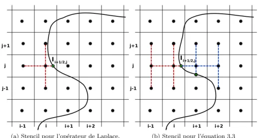
Tous ces ´el´ements nous permettent de discr´etiser sur un maillage cart´esien l’entier syst`eme d’´equations (3.1 - 3.3). Un dessin sch´ematique des stencils de discr´etisation utilis´es `a cot´e de l’interface pour l’op´erateur de Laplace et sur l’interface pour le saut de la d´eriv´ee conormale de la solution est montr´e en Figure 3.3. La condition de saut de la solution est prise en compte dans la discr´etisation des ´equations (3.1) et (3.3) comme une contribution dans le second membre.
j j+1
j-1
i-1 i i+1 i+2
I i+1/2,j
(a) Stencil pour l’op´erateur de Laplace.
j j+1
j-1
i-1 i i+1 i+2
I i+1/2,j
(b) Stencil pour l’´equation 3.3
Figure 3.3: Stencils 2D utilis´es autour de l’interface.
Evidement, en consid´erant la nature de l’approximation autour de l’interface,´ il nous faut de l’information sur la position de l’interface et sur ses normales.
En plus, les nouvelles inconnues ont besoin d’ˆetre ´enum´er´ees, afin d’assembler le syst`eme lin´eaire. Pour une bonne parall´elisation, la meilleure mani`ere de garder cette information de fa¸con efficace est d’utiliser la fonction level set pour toutes les caract´eristiques g´eom´etriques de l’interface et de stocker l’´enum´eration et la position des intersections dans une structure de donn´ees parall`ele bas´ee sur le maillage.
Deux remarques sont n´ecessaires. En premier lieu, il n’est pas toujours possible de discr´etiser la condition de transmission (3.3) avec une erreur de troncature d’ordre deux ; en effet pour cela il faut au moins deux points sur la mˆeme ligne du mˆeme cot´e de l’interface ; lorsque cela est impossible on utilise une discr´etisation avec une erreur de troncature d’ordre un. En second lieu, la condition sur le saut sur l’interface de la d´eriv´ee tangentielle peut ˆetre d´eduite de la condition sur le saut de la solution et utilis´ee pour r´eduire le nombre des points impliqu´es dans le stencil en Figure 3.3b. Diff´erents tests ont ´et´e r´ealis´es sans pour autant observer d’am´eliorations significatives que ce soit sur la pr´ecision de la solution ou sur le temps de calcul.
Les tests pr´eliminaires, r´ealis´e avec le sch´ema que l’on viens de pr´esenter dans cette section, montrent des instabilit´es dans le taux de convergence de l’erreur.
Pour cette raison on d´ecide de modifier l´eg`erement le stencil de la condition (3.3), afin de ´eviter la pr´esence de intersections trop proche l’une de l’autre.
Cette modification donne des courbes de convergence de l’erreur beaucoup plus lisses.
La g´en´eralisation de la m´ethode au probl`eme tridimensionnel est simple, grˆace `a l’approche dimension-par-dimension. Un exemple des stencils impliqu´es dans ce probl`eme est montr´e en Figure 3.4.
En ce qui concerne la parall´elisation de la m´ethode, l’utilisation de la fonc- tion level set et le stockage de l’information sur les points hors du maillage (les intersections) comme une caract´eristique des points du maillage permettent
3.2. UNE VUE D’ENSEMBLE 39
(a) Stencil pour l’op´erateur de Laplace.
(b) Stencil pour l’´equation 3.3.
Figure 3.4: Stencils 3D utilis´es autour de l’interface. Sph`eres vertes pour les intersections.
une application simple du paradigme `a m´emoire locale pour le parall´elisme, en employant la biblioth`eque PETSc. La d´ecomposition de domaine est obtenue apportant un soin particulier juste `a l’´enum´eration des intersections. Cette organisation est r´ealis´ee en cherchant ´a r´eduire le nombre de communications message passing et de garder le d´es´equilibre parmi les travaux de chaque pro- cesseurs le plus faible possible. Finalement, le code parall`ele est ´ecrit en employ- ant des instruments de codage parall`ele d´ej`a existants, presque sans s’occuper explicitement des communications.
La validation num´erique de la m´ethode est r´ealis´ee en produisant les r´esultats de convergence pour cinq diff´erents cas-test bidimensionnels et pour un simple cas-test tridimensionnel pr´eliminaire, en utilisant les impl´ementations s´equentielle et parall`ele du code. Les taux de convergence de l’erreur montrent une pr´ecision satisfaisante d’ordre deux mˆeme pour des interfaces complexes et les compara- isons avec les autre m´ethodes pr´esentes dans la litt´erature montrent une erreur absolue comp´etitive.
Les performances de scalabilit´e de l’impl´ementation parall`ele sont test´ees que ce soit pour le probl`eme bidimensionnel ou pour le probl`eme tridimension- nel, en consid´erant le cas-test le plus simple. Les r´esultats montrent un bon comportement du temps de calcul en fonction du nombre des processeurs, peu
´eloign´e du parall´elisme parfait.
Notre m´ethode est ensuite appliqu´ee pour r´esoudre les probl`emes elliptiques dans un domaine irr´egulier apparissant dans un mod`ele continu tridimensionnel de croissance tumorale, en particulier le mod`ele `a deux esp`eces de Darcy. Le mod`ele continu, au moyen d’EDP, peut traiter l’´evolution spatiale d’une tumeur pendant son d´eveloppement en fournissant des informations sur sa forme et sa position. Parmi ces mod`eles les plus complexes ne sont normalement pas adaptes pour des applications cliniques, `a cause du nombre ´elev´e de param`etres libres `a d´eterminer.
L’application actuelle doit ˆetre consid´er´ee dans le cadre des probl`emes d’iden- tification des param`etres libres d’un mod`ele. Dans ce cadre il faut r´esoudre des probl`emes inverses et trop de param`etres libres peut faire devenir cette tˆache impossible d’un point de vue du calcul. Le mod`ele `a deux esp`eces de Darcy est capable de donner une description raisonnable des ph´enom`enes. Non pas en occultant certain m´ecanismes biologiques, mais grˆace `a son nombre r´eduit de
param`etres libres par rapport `a des mod`eles plus sophistiqu´es, il peut offrir un probl`eme d’identification plus abordable.
Le mod`ele d´ecrit l’´ecoulement satur´e de trois phases dans un milieu isotope poreux non-uniforme. P, Q et S sont, respectivement, le nombre de cellules prolif´erantes (se divisant, responsables de la croissance tumorale), quiscentes et saines par unit´e de volume et les ´equations pour eux sont :
∂P
∂t +∇ ·(~vP) = (2γ−1)P+γQ (3.4)
∂Q
∂t +∇ ·(~vQ) = (γ−1)P−γQ (3.5)
∂S
∂t +∇ ·(~vS) = 0 (3.6)
o`u la vitesse~v explique la d´eformation du tissu et γ, une fonction scalaire des nutriments, d´etermine si les cellules tumorales prolif`erent ou meurent (en de- venant quiescentes). On suppose un mouvement passif. On utilise la hypoth`ese d’´ecoulement satur´e,P+Q+S= 1, et ce qui implique
∇ ·~v=γP