Paul de Kerret

D= diag (A) Diagonal matrix whose diagonal elements are equal to the diagonal elements of the square matrix A. Π⊥A(v) Orthogonal projection of the vector v over the orthogonal complement of the space spanned by the columns of the matrix A.

Saturation des bandes de fr´equence

Une mauvaise gestion des perturbations réduirait en fait considérablement les profits et pourrait même rendre ces changements contre-productifs. Par conséquent, l'importance d'un contrôle efficace des perturbations est devenue très claire à la fois dans la communauté académique et dans l'industrie (voir [4] et ses références).

Transmission ` a partir d’un transmetteur vers de mul-

La première consiste à modéliser la connaissance imparfaite du canal avec une variable aléatoire pour ensuite maximiser les performances moyennées sur ces imperfections [20]. Il a été montré dans [23] que même une estimation décorée avec l'état actuel du canal peut conduire à une amélioration des performances par rapport à un système d'estimation sans aucune information de canal pour l'émetteur.

Coop´eration de plusieurs transmetteurs

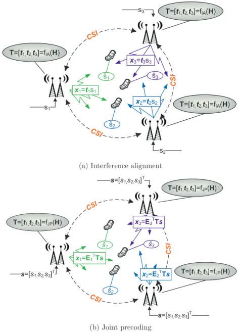
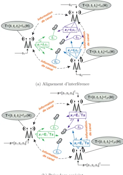
Une question particulièrement intéressante avec l'alignement d'interférence est la question de la faisabilité de l'alignement d'interférence. Ce gain est déjà présent pour l'alignement des interférences et devient encore plus important dans le cas d'un précodage conjoint.

Les d´efis de l’obtention de l’information de canal aux trans-

Information de canal imparfaite aux transmetteurs

Il demande ensuite aux TX de recevoir les informations de canal relatives à l'ensemble du groupe coopératif. Plusieurs équipes de recherche ont travaillé sur la détermination de la taille optimale des groupes collaboratifs et sur l'évaluation du coût de l'évaluation des informations sur les canaux [72, 73].

Configuration ` a information de canal distribu´ee

En particulier, nous montrons comment des gains importants peuvent être obtenus en optimisant le partage des informations de canal entre les TX. Dans la première partie de cette thèse, nous étudions le précodage à partir d'informations de canaux distribués.

Publications

Conf´erences

Paul de Kerret and David Gesbert, "A practical precoding scheme for multicell MIMO channels with partial user data sharing," in proc. Xinping Yi, Paul de Kerret and David Gesbert, “The DoF of MIMO network with backhaul delays”, in Proc.

Journaux

Paul de Kerret, Xinping Yi, and David Gesbert, “On the degrees of freedom of the K-user time-correlated broadcast channel with delayed CSIT,” in proc.

Pr´ecodage conjoint avec information de canal distribu´ee

Pr´ecodage ZF avec information de canal distribu´ee

Analyse du nombre de degr´es de libert´e (DoF)

Ainsi, le précodage AP-ZF permet d'atteindre la DoF qui serait obtenue avec la meilleure estimation disponible des deux TXs. AP-ZF consiste à définir de manière aléatoire le coefficient de précodage du TX avec l'estimation la moins précise pour que le TX avec la meilleure estimation élimine les interférences.

Analyse du pr´ecodage et des canaux de feedback

Nous considérons maintenant un exemple d'information de canal pour visualiser les résultats théoriques précédents. Ce dernier résultat fournit un critère de conception des canaux de rétroaction dans le cas d'informations de canaux distribués.

Alignement d’interf´erence avec information de canal incompl`ete 26

Analyse des sc´enarios ´etroitement faisables

Il est donc possible d'aligner les interférences en fournissant uniquement les informations relatives au plus petit canal d'interférence à chaque TX. L'algorithme consiste à former d'abord les précodeurs des TX appartenant au plus petit canal d'interférence actuellement possible.

Analyse des sc´enarios largement faisables

Nous verrons dans les simulations que la réduction obtenue de la taille des informations du canal est significative. La taille des informations de canal obtenues avec notre algorithme est de 20 alors que la taille complète est de 99.

Conclusion et nouveaux probl`emes

Saturation of the Wireless Medium

To cope with the expected saturation of available resources in the bands currently used, the architecture of the wireless networks and their transmission schemes must be reconsidered. It has then become increasingly clear that the bottleneck of future wireless networks will be interference management [4].

Downlink Multi-user Single-cell Transmission

Gaussian multiple-input-multiple-output (MIMO) channel capacity has been obtained [7, 8] and shown to be achieved by a nonlinear scheme called dirty paper coding (DPC) in which interference is subtracted on the TX side [9] . However, the performance improvement can only be achieved at the cost of an accurate knowledge of the channel state in both TX and RX [14, 15].

Multi-cell Processing

A clear advantage of TX cooperating over conventional approaches that rely on selfish interference suppression at the RXs lies in the reduced number of antennas required with each RX to ZF residual interference. In the case of three interfering TX's with two antennas, relying on RX-based interference suppression only requires three antennas at each RX to ZF-en the interference, while only two are needed when coordination via IA is possible.

The Challenges of Obtaining CSIT

• Imperfect CSIT
• The Distributed Channel State Information Setting . 41
• Contributions Presented in this Thesis
• Other Contributions
• Received Signal
• Precoding Schemes with Perfect CSIT

Paul de Kerret and David Gesbert, “Degrees of freedom of network MIMO with distributed CSI,” in IEEE Trans. We present the main principles of transmission schemes in the case where the CSI is fully known at each TX.

Figures of Merit: Average Rate, DoF, Generalized DoF

Average Rate

Similarly, the RX beamformers at all RXs are then obtained from the TX beamformers as. Note that without loss of generality (w.l.o.g.), the noise variance is normalized to one by dividing both the numerator and the denominator in (3.13) by the noise variance which amounts to integrating the noise variance into the variance of the channel. .

Degrees-of-Freedom

The general expression in (3.13) will be rewritten in simplified forms if we consider JP or IA.

Generalized Number of Degrees-of-Freedom

This dependence of the path loss with SNR allows the network geometry to be taken into account in the analysis. The generalized DoF analysis provides an approximation of the achieved capacity in the original transmission setting.

The Distributed CSIT Configuration

Distributed CSIT

This consists of using a model where the strength of any interference links is parameterized as a function of the operating SNR. Another distributed CSIT configuration that we will consider in Chapter 8 consists of letting each TX know a subset of the channel elements perfectly, with the subset of the channel elements being different for each TX.

Distributed Precoding

An example, which is studied in Chapters 4 and 5, consists of each element of ˆH(j) being taken from. A suboptimal precoding scheme consists of using a conventional precoding algorithm distributively at each TX.

Optimal Precoding with Distributed CSIT: A Team Decision

We will now reformulate the optimization problem (3.22) with the appropriate formalism to highlight how it relates to the conventional team decision problems. Finding the optimal team decision strategy is a very difficult problem as it requires solving a distributed functional optimization problem.

Summary of Objectives

Quantization for Distributed CSIT

Interestingly, this quantization scheme can be seen as insufficient in the case of distributed CSIT: The objective, which is maximized, is invariant by multiplying the codeword by a unit-rate complex number. Therefore, in the following we give an analysis of the performance of the quantization scheme (4.4) with random codes.

Distributed CSIT Model

Instead, we will use a simple model for the CSI imperfections to discuss the fundamentals of transmission. We thus also concentrate on scaling in the logarithm of the SNR of the number of quantization bits of all channel estimates.

ZF in the Two-user BC with Distributed CSIT

• Conventional Zero Forcing
• Robust Zero Forcing
• Beacon Zero Forcing
• Active-Passive Zero Forcing

As a result, we now propose a modification of the conventional ZF scheme that improves the DoF when the estimates for h1 and h2 are of different quality. However, the selection of the coefficient used for transmission at TX 1 (with the lowest CSI accuracy) remains to be discussed.

ZF in the General K-Users BC with Distributed CSIT

• Conventional Zero Forcing
• Beacon Zero Forcing
• Active-Passive Zero Forcing
• Discussion of the Results

In the proof of Theorem 4, it is in fact the scale of the interference resulting from the transmission of one current that is calculated. It then remains to determine the scale of the interference resulting from the transmission of one given data symbol.

Precoding Using Hierarchical Quantization

Hierarchical Quantization

Note that the scalar value can be sent by any of the other K−1 TXs and one scalar value must be sent for each stream. Once this is done, the decoded codeword is chosen as the representative codeword of the resulting codebook.

Conventional Zero Forcing with Hierarchical Quanti-

Active-Passive Zero Forcing with Hierarchical Quan-

The two consecutive minima come from the fact that it is not the same TX that is passive for the different currents. For K≥3, it is optimal to choose passive TX to be TXj mej=nHQ defined in (4.48), for all data streams.

Simulations

In the Two-User Case

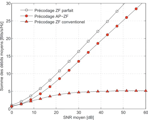
The DoF achieved with Active-Passive ZF based on hierarchical quantization is then equal to. To emphasize the DoF (i.e., the slope of the curve in the figure), we make the SNR large.

With Arbitrary Number of Users

The DoFs achieved with the different precoding schemes for this CSIT scaling matrix are given in Table 4.1. The average sum rate achieved for this institution is shown in terms of the SNR in Fig.

Conclusion

ZF with Centralized CSIT

In the case of centralized CSIT, the same estimate is received at all TXs.

ZF with Distributed CSI

Broadcast Channel with Centralized CSIT

Rate Loss Analysis

In the BC with centralized CSIT, the speed loss at user i, which we denote by ∆CCSIR,i , can be bounded at high SNR if.

Feedback Design

The following theorem provides an upper bound for the rate loss as a function of the number of return bits available to B. Setting the rate loss ∆CCSIR,i less than or equal to log2(1 +b) and solving for β yields the theorem .

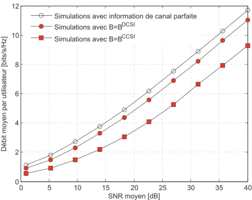
Simulation Results

We compare it to the average speed obtained using full CSIT and to the maximum allowable speed loss of log2(1 +b) = 1 bit.

Broadcast Channel with Distributed Limited CSI

Rate Loss Analysis

Starting from this proposition, we can then quantify the rate loss due to the distributed CSIT, as is done in the following theorem. In BC with distributed CSIT, if all the variances (σ(j)i )2 decrease polynomially with SNRP, the speed loss ∆DCSIR,i at userican will be upper limit at high SNR as.

Feedback Design

Note that because of this conjecture, the reaction rate obtained from (5.25) will not guarantee that the rate loss remains below the given threshold and one will have to use (5.24) to obtain a formal guarantee. Considering K larger, this response rate is approximately Klog2(K) greater than the response rate obtained in the centralized case, implying that the difference between the two expressions becomes increasingly large as the number of users K increases .

Simulation Results

Note that due to the different scale in the number of users, the loss achieved with BCCSI increases with the number of usersK.

Conclusion

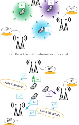
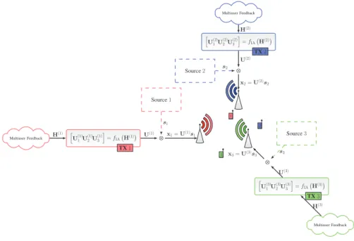
This distributed CSIT setup is depicted and compared to the centralized CSIT setup in Fig. Using the results in Section 4.1.2, the variance of the estimation error can be related to the number of quantization bits as follows.

DoF Analysis with Static Coefficients and Distributed CSI

Sufficient Condition for an Arbitrary IA Scheme

However, the accuracy of the precoder design is difficult to correlate with the accuracy of the CSIT. Furthermore, obtaining a relationship between CSIT quality and precoding accuracy is particularly difficult in the case of iterative IA algorithms.

DoF Analysis in the 3-user Square MIMO IC

It is easy to see from the continuous distribution of the channel matrices that ∀η >0,∃ε >0,Pr(Hε)≥1−η. Using Theorem 2.1 from [109] for Y⋆ and Y(j) and taking into account the expectation, we can show that for some constant γ(j)>0 is independent of the SNR P,.

Simulations

We have shown that for the closed-form 3-user IA matching scheme, the achieved DoF is greater than the worst-case accuracy of the channel estimates across the TXs. Interestingly, the lower bound at RXj is limited by the accuracy of the estimates relative to the channels of all the other RXs.

Conclusion and Outlook

Distributed CSI at the TXs

Furthermore, only the exponentially asymptotic behavior in SNR is of interest in this work, so the CSIT error distribution is not relevant here. Furthermore, only the CSI requirements in TXs are investigated and different scenarios can be envisaged for sharing channel estimates (eg, direct transmission from RXs to all TXs, sharing through a backhaul,) .

Distributed Precoding

We consider a digital quantization of the channel vectors here, but the results can easily be translated to a setting using analog feedback, since digital quantization is simply used as a way to quantify the variance of the CSIT errors [19, 112] .

Optimization of the CSIT Allocation

7.8) Therefore, an interesting problem consists in finding the minimal CSIT allocation (where minimality refers to the size in Definition 2) that achieves the maximal generalized DoF of each user:. We focus here on an “achievability result” by exhibiting a CSIT allocation that achieves the maximum DoF while having a much lower magnitude than the conventional (uniform) CSIT allocation.

Preliminary Results

A Sufficient Criterion

The maximum DoF is achieved when the velocity difference ∆R,i/log2(P) tends to zero as the SNR increases, which is the result of the proposal. However, Proposition 12 does not address the main issue of determining what type of CSIT allocation can be achieved (7.10).

The Conventional CSIT Allocation is DoF Achieving . 131

After normalization, it easily follows from (7.31) that the sufficient condition in Proposition 12 is satisfied, which completes the proof. This CSIT division provides each TX with the K channel vectors with respect to the K RXs.

Distance-Based CSIT Allocation

Distance-based CSIT Allocation

With the notations defined above, the conventional CSIT assignment given in (7.21) can be rewritten as We are now looking for a CSITB(j) assignment that provides this. 7.53) Let's write down the first coefficients in particular.

Scaling Properties of the Distance-based CSIT Allo-

Then there is no path loss interference reduction and the distance-based CSIT assignment converges, as expected, to the conven- . From the finite density assumption, there are only a finite number of RXs that satisfy this condition, so the CSIT allocation size at TXj remains bounded as Kincreases.

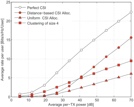
Simulations

We can observe that reducing the CSIT allocation leads to the reduction of the slope, i.e., the DoF, while the use of more feedback bits leads to a compensation of the extinction rate. This is consistent with our theoretical result that distance-based CSIT distribution leads to a finite rate offset.

Conclusion

The proposed CSIT allocation can be seen as an alternative to grouping where hard group boundaries are replaced by a smooth decrease in the strength of cooperation. The size of a CSIT distribution F, denoted by s(F), is equal to the total number of complex channel coefficients returned to TX.

Feasibility Results

• Results from the Literature
• Tightly-feasible and Super-feasible Settings
• New Formulation of the Feasibility Results
• Generalized interference channels

Condition (8.8) requires that a number of conditions be verified that increases exponentially with the size of the network. We can note that the number of conditions to test in Theorem 13 is still exponential.

IA with Incomplete CSIT for Tightly-Feasible Channels

• General Criterion
• CSIT Allocation Algorithm
• IA Algorithm for Incomplete CSIT Allocation
• Example of Tightly-feasible Configuration

In the following we assume that the beamformers of TXs and RXs within this sub-IC are fixed and complete all IA contents within this sub-IC. By inspection of the CSIT allocation algorithm, the CSIT allocations of all TXs included in STX(j) are included in the CSIT of TXj.

Interference Alignment with Incomplete CSIT for Super-Feasible

CSIT Allocation Algorithm

We also define the number of RXs and the number of TXs actually in the generalized IC QK. The closely feasible sub-ICs are obtained by following similar steps as in the algorithm in section 8.3.2.

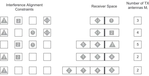
Toy-Example of the Incomplete CSIT-Algorithm in

Any antenna can be removed and the policy chosen in the algorithm is to remove the antenna on the TX with the smallest number of antennas if there is at least one TX left [Cf. The IA algorithm for incomplete CSIT sharing resulting from this CSIT assignment is symbolically depicted in Fig.

Simulations

Tightly-Feasible Setting

Since this setting is firmly executable, we can perform the CSIT assignment for firmly executable ICs described in subsection 8.3.2, which returns the CSIT allocation. The reduction of 60% of the feedback size (Cf. Subsection 8.3.4) therefore comes for nothing, which makes it particularly interesting in practice.

Performance Evaluation of the CSIT allocation Algo-

For reference, we also show the average size of the full (conventional) CSIT allocation. If more than 12 antennas are available, each additional antenna is used by the heuristic algorithm to reduce the size of the CSIT map.

Discussion

The focus of this thesis has been the analysis of multi-antenna cooperation schemes in the case of imperfect CSI sharing between TXs. The focus of the second part of this thesis was the optimization of the spatial allocation of CSIT.