In the setting of the Holmgren theorem, local estimates of unique continuation of the form (1.4) were proved by John [Joh60]: they are of Hölder type, i.e. in the situation of the Hörmander theorem it is proved by Bahouri [Bah87] that Hölder stability always holds locally.
The wave and Schrödinger equations
In the former estimate, Λ should be considered as the typical frequency of the initial data. The solution of the non-homogeneous boundary value problem is rejected in the sense of transposition, see [Lio88a].
Quantitative unique continuation for operators with partially analytic coecients
Let us now consider the example of operators P of the main symbol of the form p2(x, ξ) =Qx(ξ), where Qx is a smooth family of real quadratic forms such that Qx(0, ξb) is defined on Rnb. We have chosen not to present this more general result here for the sake of presentation.
Idea of the proof
In Section 6, we specify our general result in the case of the wave and Schrödinger equations. As for the unique (qualitative) continuum, there is no need to prove quantitative estimates to the limit.
The Carleman estimate
Above and below, there is distance to the Euclidean distance in Rn, RorRna or the Riemannian distance of (M, g). Rna) we dene a dneghborhood ofK city. We denote by F the Fourier transform in all variables, Fa only in the variablesnexa∈Rna.
Regularization of cuto functions and Fourier multipliers
We now discuss in more detail the basic properties of this regularization process only in the second case (the first case can be seen as the special situation na= 1, nb= 0). Furthermore, the function fλ can be expanded as a whole function in variablexa with. whereζa2=ζa·ζa=|Reζa|2− |Imζa|2+ 2iReζa·Imζa is the real inner product) with uniform bound.
Some preliminary estimates
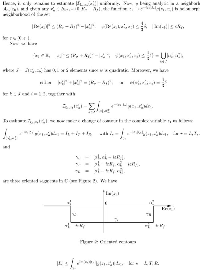
Functional being real analytic in the variable in a neighborhood of the compact set BRna(0, Rσ), there exists Rf >0 such that it can be expanded analytically in a neighborhood ofza∈BRna(0, Rσ+Rf)+iBRna(0 , Rf), uniformly forxb∈Kb. The constants in the exponentials do not depend on α, since they are functions only of ψ, Rσ, Rf, Kb. bg)(ξa, xb) finally completes the proof of the lemma.
Step 2: Using the Carleman estimate
B1 consists of terms where there is at least one derivative on χδ,λ(ψ) and none on σ2R and χeδ(ψ). B3 consists of terms where there is at least one derivative on σR,λ and none on χδ,λ(ψ), χeδ(ψ) and σ2R. Proving the evaluation of the last term in (3.18) consists of successive evaluation of the related expressions with the generic expressions B±, Bˇ2,Bˇ3, Bˇ4; then the final estimate follows, since the LHS (3.19) is bounded by the final sum of such terms.
In the special case of termspα(xb)∂α, i.e. some coefficients independent onxa, we can have some better estimates uniform in the magnitude of pα. Furthermore, ifpα is only analytic inxa and bounded inxb, all estimates of the commutator remain valid. Now we are ready to apply the Carleman estimate (3.12) to obtain the estimate of the next lemma.
We also have to estimate the termeτ(ψ−d)P σ2RσR,λχδ,λ(ψ)χeδ(ψ)u: we have that. 3.28) where we have used Lemma 2.13 several times for χδ,λ(ψ) or some of its derivatives of order less than m−1.
Step 3: A complex analysis argument
The proof essentially consists of running a scaling argument to remove the µ parameter and then applying Lemma B.2. The Local Estimate of Theorem 3.1 only provides information about the low-frequency part of the function. They are intended to describe how information about the low-frequency part of the solution can be derived from one sub-region to another.
Now we list some general properties of the relation E, which actually hold without using any assumption on the setΩand the operatorP. Taking the weakest of the constants C, κ0, µ0 given by applying the denition for any, it gives. We have Uei ⊂W for alli∈I, so Property 2 and then Property 1 of the previous Lemma gives(Vj)j∈JEW which implies (Vj)j∈JCU sinceW bU.
Then property 5 of the previous lemma gives (Vi)i∈I E(Uei)i∈I, which gives (Vi)i∈IC(Ui)i∈I by negation.
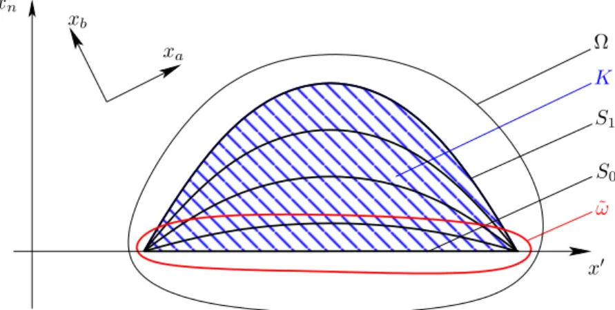
Semiglobal estimates along foliation by graphs
Note that in the above proofs we have omitted to specify each time the constraint µ≥µ0. This gives that for any ωe⊂Ωe neighborhood of S0 there exists an open setUe neighborhood of K (which we can impose included in Ωe), so we have the estimates. Now we come to the proof of the main result of this section, namely Theorem 4.7.
Noting the proof of Theorem 4.7, we have for each k∈J0 N−1Kandi∈Iεk. where we consider the union S. Now we will use an abstract iteration argument, so for j ∈ J1, NK=J and i∈Iεj: we set the following notations. By Corollary 4.6, choosing therεij and ρεij ≤ρεj implies Ui,jCVi,j. Furthermore, we have ωi,jbUi,j and Lemma 4.8 can be written as Vi,k+1bh U0∪S. We can now use the following iteration proposition, which we will prove later. Since U is a neighborhood of K by the coverage property (4.12), this completes the proof of Theorem 4.7, up to the proofs of Lemma 4.8 and Proposition 4.9.
IAk) Note that using property 4 of Proposition 5 and since we can choose W0 with U0bW0bV0 and ωi,jbUi,j, we have.
Semiglobal estimates along foliation by hypersurfaces
The proof is exactly the same as that of Theorem 1.10/4.7 except that local uniqueness evaluations are performed on Ω. But since Φ is a homeomorphism, it implies the existence of rex and Rfx (which can still be chosen small enough) such that Φ−1. The geometric part of the proof of Theorem 1.10/4.7 is then exactly the same, performed on Ωe, i.e.
Once the geometric part is done, the iteration process, which is performed in Ω, is exactly the same by replacing each geometric term by the example in Ω (for example Φ−1h. Assume that the variables xare tangent to the boundary, and that the functions satisfies Dirichlet boundary conditions, we prove a counterpart of the local estimate of Theorem 3.1 for this boundary value problem This situation is of particular interest for the wave equation for which xa is the time variable, which is always tangent to the boundary of cylindrical domains .
For simplicity, we further assume that the operator principal symbol for Pi is independent of the thexa variable (otherwise we would have to assume that the coecients of P are analytic with respect to xa).
Some notation
In this section we will consider a specific class of operators as described in Remark 1.9, that is, with symbols of the form p2(x, ξ) =Qx(ξ) where Qx is a smooth family of real quadratic forms. For k ∈N, the norm k·kk,+ will denote the classical Sobolev norm on Rn+ and k·kk,+,τ the associated weighted norms, that is.
The Carleman estimate
In conclusion, if is a linear operator from Hk to Hl of norm C that sends(T)∩Hk to ker(T)∩Hl, then, extends to a linear operator from Hk(Rn+)toHl(Rn+) and we have. The proof of this theorem relies on a Carleman estimate that interpolates between the elliptic limit Carleman estimates of Lebeau and Robbiano [LR95] and the partially analytic Carleman estimates of Tataru [Tat95] (see also [Hör97]). For suchτ, these two terms can be absorbed into the left side of the inequality.
The second term has the same form as the right-hand side of the Carleman estimate, up to and including change of d. To prove Theorem 5.2, we define the conjugate operator Pψ=eτ ψP e−τ ψ=P(x, D+iτ ψ0), and also Pψ,ε the conjugate ofPψ with respect to e−2τε|Da|2, which i.e. like that. 5.6) Since P is independent of onxa, it is. Now that we've done the exact calculations, let's make some guesses about the symbols of the commutator's inner part.
The idea is to transfer the assumption of the positivity of the solid symbol to some positivity of the tangent symbol, which will then allow the use of tangential Gårding.
The local quantitative uniqueness result
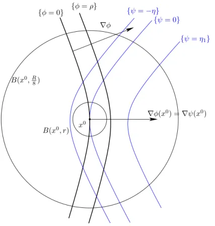
The proof of the local quantitative uniqueness will then be essentially the same as in the boundless case. The following Proposition is the counterpart, in the limiting case, of the end of the first step in Section 3 (thus containing the geometric part of the proof of the local uniqueness result). Let φ be a function in a neighborhood of x0 in Rn such that φ(x0) = 0, and {φ= 0} is a C2 strongly pseudoconvex oriented surface atx0 in the sense of Denise 1.6.
Finally, the geometric statement of Item 1 arises from the application of Lemma 3.4 in the geodetic coordinates. Assume that there is a function φ defined in a neighborhood of x0 in Rn such that φ(x0) = 0, and {φ= 0} is a strongly pseudoconvex oriented surface atx0 in the sense of Denition 1.6 and such that φ0xn(x0) >0. In addition, we have added the potential V with respect to the general case; we also need to check that it is painless in the trial.
Proposition 5.10 gives the corresponding convex ψ, a second degree polynomial in the variable x that satisfies the desired geometric conditions, together with the Carleman estimate (5.4).
The semiglobal estimate with boundary
We complete the proof as in Theorem 1.10 once Theorem 4.7 is proved, taking into account Remark 5.1. It is clear that the proof of the Theorem involves quite a number of applications of Theorem 5.11 and 5.12. Indeed, the proof scheme of Theorem 4.7 involves only a whole number of applications of the geometric propagation of the property C.
We now give applications of the above main results, namely theorem 1.10 and in the case of limit theorem 5.13 to the wave and Schrödinger operators. The proof each time consists of using the quantitative estimates of Theorem 5.13 and then using energy estimates to relate the energy to the initial data and the source term. The uniform dependence with respect to time-independent lower-order expressions follows from the fact that we use only a ninth number of times Theorem 5.13.
With Theorem 6.3 we now conclude the proof of Theorem 6.1, using energy estimates to relate k(u0, u1)kH1.
The Schrödinger equation
As in the case of the wave equation, the preceding theorem is a combination of the following theorem and energy estimates for the Schrödinger equation. In the case when R = W0∂t+W1· ∇+V does not depend on t, the dependence on the size of the coefficients of R remains the same as theorem 6.3. The proof is quite similar to that for the wave equation, so we only outline the main steps of the proof.
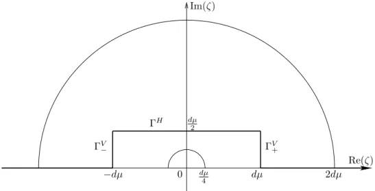
We use the same coordinate diagrams as given in the proof of Theorem 6.1 for the wave equation. The dependence on the lower order term R follows in the same way as for the wave equation. The following is a version of the Phragmén Lindelöf principle for subharmonic functions in a sector of the complex plane.
We prove this as a consequence of the maximum principle for subharmonic functions in bounded domains.