[PENDING] Quantum slit diffraction in space and in time of a Gaussian wave packet and semi-classical approximation

HAL Id: hal-00875304

https://hal.archives-ouvertes.fr/hal-00875304v1

Preprint submitted on 21 Oct 2013 (v1), last revised 14 Feb 2014 (v3)

HAL is a multi-disciplinary open access archive for the deposit and dissemination of sci- entific research documents, whether they are pub- lished or not. The documents may come from teaching and research institutions in France or

L’archive ouverte pluridisciplinaire HAL, est destinée au dépôt et à la diffusion de documents scientifiques de niveau recherche, publiés ou non, émanant des établissements d’enseignement et de recherche français ou étrangers, des laboratoires

Quantum slit diffraction in space and in time of a Gaussian wave packet and semi-classical approximation

Mathieu Beau, T.C. Dorlas

To cite this version:

Mathieu Beau, T.C. Dorlas. Quantum slit diffraction in space and in time of a Gaussian wave packet and semi-classical approximation. 2013. �hal-00875304v1�

Quantum slit diffraction in space and in time of a Gaussian wave packet and semi-classical approximation

Mathieu Beau and Tony Dorlas

School of Theoretical Physics, Dublin Institute for Advanced Studies, 10 Burlington Road,Dublin 4

(ΩDated: October 21, 2013)

Abstract

We revisit the famous problem of quantum slit diffraction of a three-dimensional Gaussian wave packet, taking into account the diffraction in time phenomenon for a reflective or absorbing slit.

We first recall the theory of diffraction in space and in time to give an explicit integral formula for the single-slit propagator (for a two-dimensional aperture) assuming that the time of opening the aperture coincides with the time of emission of the particle. Then we derive a semiclassical expression for the amplitude when the parameter µ=m|r|²/(~t) is large, where ris the position of the particle with mass m detected on the screen at the time t. We also give corrections to the law giving the distance between two fringes in the Fraunhofer regime when the distances of the apparatus in the propagation direction are large compared to the size of the aperture of the slit. To conclude, we discuss the phenomenological consequences and we give a new perspective to investigate the quantum diffraction phenomenon particulary for the cold atom slit experiment.

CONTENTS

I. Introduction 2

II. Diffraction in space (DIS) and in time (DIT) of a localized wave packet 5

A. Basic set up 5

B. One-dimensional diffraction in time of a localized wave packet 8 III. One-slit diffraction model and its semiclassical approximation 10 A. Single-slit diffraction of a narrow Gaussian wave packet 11

B. Semiclassical limit of the one-slit propagator 13

IV. Semi-classical approximations for the slit experiment 18

A. The truncation approximation 19

B. The fourth-order approximation in the Fraunhofer regime 20 C. Criterion for the validity of the fourth-order approximation 22

V. Discussion 24

A. General remarks 24

B. Ultracold atoms slit experiment under gravity 25

C. Conclusion 28

VI. Appendices 29

A. Appendix 1: The truncation approximation for the quantum-multi-slit diffraction

problem 29

B. Appendix 2: Derivation of the one-point source propagator 31

C. Appendix 3: Diffraction patterns 32

References 33

I. INTRODUCTION

The quantum slit diffraction experiment of electrons was first realized experimentally in 1961 by C. J¨onsson, see¹ and², but the first experimental proof of the quantum diffraction for individual electrons was shown in the seventies by O. Donati, P. G. Merli, G. P. Missiroli

and G. Pozzi,³,⁴ using electron biprisms and later independently by A. Tonomura, J. Endo, H. Ezawa, T. Matsuda and T. Kawasaki⁵. The quantum diffraction phenomenon has been interpreted via the famous thought experiment imagined by Richard Feynman in⁶. We mention that this double slit experiment has recently also been done experimentally⁷ in a situation where the probability distribution for individual electron on the screen was observed (statistically) while varying the position of a mask hiding one, two or none of the slits. In addition, nano-slit electron experiments were recently performed, see for example⁸. Futhermore, slit experiment were carried out with neutrons, see⁹ and the references therein, ultracold atoms¹⁰ and with heavy molecules such as C60, see¹¹.

In¹², Feynman also treated in detail a quantum slit diffraction model using the path integral formalism to compute the quantum slit propagator. The model consists of a one- dimensional slit appearing in the motion of an electron at a timeτ > t0 = 0 and then removed instantaneously, the electron striking the screen at a time t > τ. Actually, this means that the motion of the electron from the source to the screen consists of two independent motions, the first from the source to the slit and the second one from the slit to the screen. Under this hypothesis, the quantum propagator for the single-slit system can be written as a product of the free propagator in thex-direction orthogonal to the slit and the propagator along the one-dimensional slit axis z: see¹³ and¹⁴ for pedagogical presentations of this model. This so- called “truncation approximation”¹⁹ is convenient and valid under certain conditions. First, we suppose that the particle passes through the aperture at the classical time τ = tc = D/vx = (D/x)t, where D is the distance between the emittor and the center of the slit, x is the distance between the emittor and the screen, and vx = x/t is the classical velocity related to the wave length λ by the de Broglie relation λ ≈2π~/(mv_x) = 2π~t/(mx). Here we assume v ≈vx because we have a ≪x, wherea is the size of the slit, and we take z ≪x where z is the position of the particle detected on the screen. Moreover, we also assume that the motion along the x-axis is classical whereas the one parallel to the screen (in the z direction) is quantum. The main aim of this article is so to find the condition justifying the latter assumption, i.e. the classical behavior of the particle along the x-axis, independently of the fact that we consider the aperture of the slit to be relatively small, and also to give a correction to the single-slit propagator formula and to analyse the higher-order correction to the probability density function for different regimes.

At this stage, we should mention that another curious quantum diffraction phenomenon

was imagined in 1952 M. Moshinsky¹⁵. He showed that for a monochromatic plane wave moving along the one-dimensional line, if a perfectly absorbing screen is placed at a fixed position on the axis at the times 0 < t < t₁ and is removed at the time t₁, the probability density function would be similar to the one observed for the diffraction in space by a half- plane. By analogy, therefore, we call this phenomenon diffraction in time, and it was first observed experimentally in 1997 by the cold atom team of the Kastler Brossel Institute in Paris, see¹⁶. In the mean time, the problem of diffraction in both space and time of monochromatic plane waves for a perfectly reflective slit-screen was treated in¹⁷. They used the Green’s function method, giving the general solution of the diffusion equation¹⁸ in the half-space delimited by the plane of the slit with given boundary conditions. Recently, in¹⁹, another approach was suggested to treat the space and time diffraction problem but for a Gaussian wave packet and for a perfectly absorbing screen.

In this article, we use the Brukner-Zeilinger approach¹⁷to revisit the quantum slit diffrac- tion of a Gaussian wave packet. In Section II, we introduce the following model. Consider a particle, modelled by a three-dimensional Gaussian wave packet of widthσ, which is emitted at the time t0 = 0 from the position x0 < 0, y0 = 0, z0 = 0. The aperture of the slit is closed until it is opened at the time t1 ≥0 after which the wave packet propagates from a rectangular aperture of the slit (centered atx= 0) to a screen (centered atx >0) where the position (y, z) of the particle is detected at a timet > t₁. In Section III, we derive an explicit integral formula for the single-slit propagator (for a rectangular aperture) for all boundary conditions on the plane of the slit, in the case where the times of emission of the particle and of opening of the slit coincide: t₁ = t₀ = 0. After that, we will show that there is a semiclassical transition, when the parameter µ=m|r|²/(~t) is large, where ris the position of the particle detected on the screen at the time t. We will also interpret the semiclassical propagator formula as a sum over classical paths going through the aperture at different times depending on the position at which the particle passes through the slit. To illustrate the semiclassical transition we calculate numerically the probability density function for a narrow Gaussian wave packet , σ∼0. In Section IV we give a correction to the truncation approximation propagator in the Fraunhofer regime when the dimensions of the aperture are small compared to the distance between the slit and the screen. Then we give a formula for the shift in the distance between two successive minima of the probability distribution function compared to the classical result. In the last section, we will discuss an experimental

perspective to the diffraction pattern for a relatively large aperture of the slit.

II. DIFFRACTION IN SPACE (DIS) AND IN TIME (DIT) OF A LOCALIZED WAVE PACKET

The aim of this section is to recall the theory of diffraction in space and time and to give a general solution to the Schr¨odinger equation for an initial Gaussian wave packet on the half space delimited by a plane. The purpose of this study is to give the physical ingredients and the mathematical tools to treat the problem of the slit diffraction beyond the truncation approximation. The latter main problem will be explored in the subsequent sections.

A. Basic set up

The diffraction-in-time experiment consists of opening a shutter at position x1 = 0 at a timet1 ≥0 and observing the particle at a pointx >0 after the opening timet−t1 >0. In¹⁵ as well as in¹⁷, the wave at the source is considered to be a monochromatic plane wave. Here we consider, as in¹⁹, a localized wave packet (Gaussian), but we follow the method developed in¹⁷ to find the general solution. To understand the difference between the localized wave packet versus plane wave, we notice that the phase of the wave is non-linear in space and in time (for one dimension ϕt(x) = ^mx_2~t²) and so the coordinate and time of emission of the localized wave has to be taken into account (which is not the case for a plane wave since the phase is linear in time, ϕt(x) = kx− ^~2m^k2t). Thus, for the truncation approximation model, the half-plane diffraction amplitude for a Gaussian wave packet is given by Fresnel integrals (see¹⁴) whereas for a plane wave this amplitude is given by the Fourier transform of the shape of the aperture (for example of a two dimensional gate function for a rectangular aperture). We will see that the result for the space diffraction of a localized wave packet by an half-plane is actually similar to the so-called “diffraction in time”.

To give a general solution of the diffraction in space and time problem, we first write the Schr¨odinger equation for the wave function of the particle moving in the apparatus:

~²

2m∇²ψ(r, t) +i~^∂

∂tψ(r, t) = 0

ψ(r, t) = 0 for x > x1 and t < t1, and ψ(r1, t) =φ(r1, t) for t > t1. (1)

Here we fixed the initial condition in the half-plane to be zero at times t < t1 and inhomo- geneous Dirichlet boundary conditions on the plane of the slit x =x1 for t > t1. In¹⁷, the boundary condition is taken to be a monochromatic plane wave φ(r₁, t) = e^−iω0t, whereas here we will consider a localized wave packet (Gaussian).

We would like to write the solution of (1) using the point source method by computing the Green function solution of the equation:¹⁸

~²

2m∇²G(r, t,r^′, τ) +i~∂G(r, t,r^′, τ)

∂t =i~δ³(r−r^′)δ(t−τ) (2) with the causality conditions:

G(r, t < τ,r^′, τ) = 0, ∇G(r, t < τ,r^′, τ) = 0 (3) The free Green function for infinite volume with the conditions (3) is:

G₀(r−r^′;t−τ) =

m 2iπ~(t−τ)

3/2

e^im|

r−r′ |2

2~(t−τ) θ(t−τ) (4)

Here we recall the solution of the Schr¨odinger equation (1) and we refer the reader to¹⁷ and¹⁸ for more details:

ψ(r, t) = Z

V

d³r^′G(r, t,r^′, t1)ψ(r^′, t1) + i~

2m Z t

t1

dτ Z

∂V

dS1[G(r, t,r₁, τ)∇^r1ψ(r1, τ)−ψ(r1, τ)∇^r1G(r, t,r₁, τ)] (5) Here∂V is the boundary of the half-plane, i.e. the 2-dimensional surface x=x₁.

In the following, we denote by r_⊥ = (y, z) the coordinates in the plane orthogonal to the x-axis and r_⊥,1 = (y1, z1) the same at the shutter. We consider general homogeneous conditions for the Green function:

G(r, t,r₁, τ) =λ1G0(x−x1,r_⊥−r_⊥,1;t−τ) +λ2G0(x+x1,r_⊥−r_⊥,1;t−τ) . (6) By a direct calculus we have :

∂x1G(r, t,r₁, t1)|^x1=0 = (−λ1+λ2)im

~ x

t−τG0(x,r_⊥−r_⊥,1;t−t1) (7) In particular we have the following special cases:

(i) for λ1 = 1λ2 =−1, we have the homogeneous Dirichlet conditions, G(r, t,r₁, τ)|^x1=0 = 0 (ii) forλ1 = 1λ2 = 1, we get the homogeneous Neumann conditions, ∂x1G(r, t,r₁, τ)|^x1=0 = 0

(iii) for λ1 = 1λ2 = 0, we get the free Green’s function G(r, t,r₁, τ) =G0(r−r₁;t−τ)

Notice that the volume is the half-space to the right-hand side of the shutter V = [0,+∞)×R×R and we consider that the initial wave function vanishes in this domain ψ(r^′, t1) = 0, if x^′ >0, with r^′ = (x^′, y^′, z^′). Then by (5), we get the following solution :

ψ(r, t) = i~ 2m

Z t t1

dτ Z

∂V

dS1[G(r, t,r₁, τ)∇^r1ψ(r1, τ)−ψ(r1, τ)∇^r1G(r, t,r₁, τ)]_x1=0. (8) Note that dS₁ is the elementary boundary surface vector orthogonal to the plane at the point r₁ and pointing outward of the volume (i.e. dS1 =−dy1dz1e_x). On the surface of the aperture ∂V, we consider that after opening the shutter, the wave function is a Gaussian wave packet which was emitted at time t0 = 0, and therefore given by the following wave function at each point r₁ ∈∂V:

ψ(r₁, τ) = Z

R³

dR G0(r₁−R;τ)φ(R,0)θ(τ−t1), (9) where the normalized Gaussian wave packet φ is given by:

φ(R,0) = 1

(2πσ²)^3/4e^−|

R−r0|2

4σ2 , (10)

where R = (X, Y, Z) and so X denotes the coordinate along the x-axis. The probability density for the initial wave packet is such that |φ(R,0)|² →δ³(R−r^′) when σ →0. In the sequel we will consider the case thatσis small compared to the distance|x1−x0|between the positionx0of the center of the Gaussian of the wave packet and the position of the shutterx1.

Remark. To relate the conditions (9) to the condition in¹⁷, let us rewrite the initial condition at the emission of the wave packet as a Gaussian distribution of plane waves:

φ(R,0) = Z

R³

dk ϕ^k(r₀−R,0)e^−σ22k2 (11) where φ^k(r0−R,0) = e^ik·(r0−R). Then, if we choose the same boundary condition on the surface (x1 = 0, y1, z1) for the plane waves defined just above as the one considered in¹⁷:

ϕ^k(r₀−R, τ) =e^{ik·(r1−r0)}e^−iωτθ(τ−t₁) (12) with the dispersion relation ω = ^~k_2m², we directly get (9) from (12) and (11). Notice that in (10) we have arbitrarily chosen the initial wave vector to be zero, but we could generally

set:

φ^k₀(R,0) = 1

(2πσ²)^3/4e^−|

R−r0|2

4σ2 e^{ik0·(r0−R)} , (13)

where the initial wave vector isk₀. However, in the following, we will assume thatσ is close to zero and so there will not be a privileged initial wave vector, which is why we takek₀ =0 in the sequel.

By (8) and (9), we get the following formula ψ(r, t) =

Z

R³

dR K(r, t,R,0|∂V, t0)φ(R,0) (14) where the propagator is defined by:

K(r, t,R,0|∂V, t1)≡ i~

2m Z t

t1

dτ Z

∂V

dS1·[G(r, t,r₁, τ)∇^r1G0(r1−R, τ)−G0(r1−R, τ)∇^r1G(r, t,r₁, τ)]_x1=0 (15) Remark. To avoid confusion, we stress that (14) is different from the volume integral term of the general solution (5): we have just rewritten (8) using the expression (15) and the integral (9).

Since

∇^r1G0(r1−R, τ) = im

~

r₁−R

τ G0(r1−R, τ)

∇^r1G(r, t,r₁, τ) = im

~

−λ1

r−r₁ t−τ +λ2

r+r₁ t−τ

G0(r−r₁, τ) we get:

K(r, t,R,0|∂V, t₁) =

−1 2

Z t t1

dτ Z

∂V

dS1·

r₁−R

τ (λ1+λ2) +λ1

r−r₁ t−τ −λ2

r+r₁ t−τ

x1=0

G0(r−r₁, t−τ)G0(r1−R, τ)|^x1=0

(16) B. One-dimensional diffraction in time of a localized wave packet

Consider the one-dimensional diffraction-in-time problem for a Gaussian wave packet emitted at x0 <0 at the time 0. By similar arguments to those leading to (16), we get, for

general boundary conditions, the following propagator:

K(x, t, X,0|x1 = 0, t1) = Z t

t1

dτ −X

τ η1+ x t−τη2

G0(x, t−τ)G0(−X, τ) (17) where we put

η1 = 1

2(λ1+λ2) (18)

η2 = 1

2(λ1−λ2). (19)

Notice that choosing η ≡η2 = 1−η1 , η ∈C and taking t1 = 0, a direct calculation shows that the integral in (17) is equal to G₀(x−X;t) and so it gives the general solution for the free particle motion, see¹⁹. Now, if we takeη = 1/2 (i.e. λ2 = 0 andλ1 = 1) then we get the free boundary condition corresponding to the perfectly absorbing shutter-screen condition.

The correct solution for t1 >0 is equivalent to the Moshinsky solution:

K⁽⁰⁾(x, t, X,0|x1 = 0, t1) = 1 2

Z t t1

dτ

−X

τ + x t−τ

G0(x, t−τ)G0(−X, τ) (20) which is easily evaluated (see¹⁹):

K⁽⁰⁾(x, t, X,0|x1 = 0, t1) =G0(x−X;t)

"

1 + 1

2erfc xt1

t +Xt−t1

t

s mt 2i~t1(t−t1)

!#

(21) Hence, by (17), we get the propagator for general homogeneous boundary conditions,

K^(G)(x, t, X,0|x1 = 0, t1) =λ1K⁽⁰⁾(x, t, X,0|x1 = 0, t1)−λ2K⁽⁰⁾(x, t,−X,0;x1 = 0, t1) . (22) similar to the case of a monochromatic plane wave¹⁷. For λ1 =−λ2 = +1 we get Dirichlet boundary conditions whereas forλ1 =λ2 = +1 we have Neumann boundary conditions.

The solution of the one-dimensional Schr¨odinger equation for the perfectly absorbing shutter-screen is obtained by inserting (20) into the one-dimensional version of (14):

ψ(x, t) = Z +∞

−∞

dX K⁽⁰⁾(x, t;X,0|x1 = 0, t1)ψ(X,0)

= Z +∞

−∞

dX K⁽⁰⁾(x, t;X,0|x1 = 0, t1)e^−(X−x0)

2 4σ2

(2πσ²)^1/4. (23) In particular, if we assume thatσ ≪ |x0|, we get that ψ(x, t)≈(8πσ)^1/4K⁽⁰⁾(x, t;x0,0|x1 = 0, t1).

Notice that the explicit solution (21) forσ≪ |x0|is similar to the explicit formulas giving the propagator and the wave function for the half-plane diffraction problem in the truncation approximation¹⁹. So both diffraction phenomena are analogous and this is why we use the term “diffraction in time” even for the localized wave packet. In the next subsection, we will see that we can also construct an analogous Moshinsky shutter problem for a localized wave packet and show the equivalence between both approaches for general homogeneous boundary conditions.

III. ONE-SLIT DIFFRACTION MODEL AND ITS SEMICLASSICAL APPROXI- MATION

In the last section, we gave the theory of diffraction in space and time for a wave packet and we furnished the general solution of the Schr¨odinger equation for an initial Gaussian wave packet passing through an aperture which is opened at a time t1 ≥t0 = 0, wheret0 is the time of the emission of the initial wave packet. We have also seen that we can interpret this phenomenon as a diffraction in time by analogy with the diffraction in space. However, since the main problem of this article is to derive a formula for the slit diffraction problem, where the aperture is not assumed to be small compared with the distance between the slit and the screen (and the slit and the source), we would like to interpret the so-called diffraction in time phenomenon in a different way, where the apparatus is fixed in time (no shutter) and the problem is stationary. In this section, we apply the theory developed in the previous section to the slit diffraction problem and give a geometric interpretation for the propagator. We first give an explicit formula for the propagator with general boundary conditions, then give its semiclassical expression and comment on the results. We also give numerical results for intensity patterns on the screen in the delta limit σ → 0 for the Dirichlet, Neumann and free boundary conditions and comment on the differences. In the next section, we will use the semiclassical formula of the propagator to give corrections to the truncation approximation model.

A. Single-slit diffraction of a narrow Gaussian wave packet

We consider the slit Ωa,b≡ {x1 = 0}×[−b, b]×[−a, a], and assume that the shutter is open at the time t1 = 0. The dynamics of the particle obeys the Schr¨odinger equation (1) and the boundary conditions are given by (9), (10). Here we consider the general homogeneous boundary conditions (6). By (16) we get the following formula for the propagator:

K^(a,b)(r, t,R,0) = Z t

0

dτ Z a

−a

dz1

Z b

−b

dy1

−X

τ η1+ x t−τη2

G0(r−r₁, t−τ)G0(r1−R, τ) (24) The integral over the time of the one-point source propagator (for every r₁ ∈∂V fixed) can be evaluated explicitly. The resulting formula will be analyzed in the semiclassical limit using the stationary phase approximation method which yields a semiclassical interpretation of the propagator. The one-slit propagator is then given by an integral of this one-point source propagator over the aperture of the slit. Finally, the wave function on the screen at time t is given by (14), where we consider an initial narrow Gaussian wave packet (10) of width σ which is small compared to the distance between the center of the Gaussian and the slit and also to the size of the aperture:

σ ≪ |r₀|, a, b.

By (14) we then have the following approximation:

ψ(r, t) = (8πσ²)^3/4 Z

R³

dR K^(a,b)(r, t,R,0)e^−|

R−r0|2 4σ2

(2πσ²)^3/2

≈(8πσ²)^3/4K^(a,b)(r, t,r₀,0), when σ∼0 (25) Therefore, in the sequel we will take R = r₀ in (24) since the final wave function is just proportional to the one-slit propagator.

Remark. In the limit σ →0, we would like to give a formula for the probability density for the particle to be at the pointr on the screen at the time t. This has already been done for the truncation approximation, see¹⁴and Appendix 1, and the general idea here is similar.

It is important to realize that |ψ(r, t)|² represents the non-normalized wave function at the point r on the screen at the time t and so, to get the probability, we have to divide by the

total mass on the screen:

M ≡ Z +∞

−∞

dy Z +∞

−∞

dz |ψ(r, t)|² .

For the truncation approximation model, the particle is assumed to pass through the slit at the classical timet_c (given by a linear relation between tand the distances along thex-axis).

Hence, the total mass passing to the right side of the plane of the slit is equal to the total mass on the screen:

Z b

−b

dy1

Z a

−a

dz1 |ψTrunc(r1, tc)|² = Z +∞

−∞

dy Z +∞

−∞

dz |ψTrunc(r, t)|² (26) However, in our model there is no similar conservation equation to (26) since we do not know the exact time when the particle passes through the aperture. Hence, the expression for the probability density at the point r and at the time t has to written as

P(r, t) = 1

M|ψ(r, t)|² → 1

Ω|K^(a,b)(r, t,r₀,0)|², when σ →0 (27) where Ω≡R+∞

−∞ dyR+∞

−∞ dz|K^(a,b)(r, t,r₀,0)|².

The formula (24) can be rewritten as an integral over all points r₁ = (x1, y1, z1) in the slit (i.e. y₁ ∈[−b, b] and z₁ ∈[−a, a]):

K^(a,b)(r, t,r₀,0) = Z a

−a

dz1

Z b

−b

dy1K(r, t;r₀,0|r₁), (28) where we have defined the three-dimensional one-point source propagator:

K(r, t;r₀,0|r₁)≡ Z t

0

dτ −x0

τ η1+ x t−τη2

G0(r−r₁, t−τ)G0(r₁−r₀, τ) . (29) We want to give an explicit formula for the one-point slit propagator (29). For a detailed calculuation we refer the reader to Appendix 2. The result is the following explicit formula:

K(r, t;r₀,0|r₁) = At(r;r₀|r₁)e^{iϕt(r;r0|r1)} (30) where the phase is given by

ϕ_t(r,r₀|r₁)≡ m

2~t(|r−r₁|+|r₁−r₀|)² (31) and where the amplitude is given by a linear combination of the Neumann and Dirichlet amplitudes:

At(r,r₁−r₀)≡η1A^(N)_t (r,r₁−r₀) +η2A^(D)_t (r,r₁−r₀). (32)

The Neumann part is given by:

A^(N_t ⁾(r,r₀|r₁) = −x0

(2iπ~t/m)^3/2 m

2iπ~t

(|r−r₁|+|r₁−r₀|)²

|r−r₁||r₁−r₀|² + 1 2π|r₁−r₀|³

(33) and the Dirichlet part by:

A^(D)_t (r,r₀|r₁) = x (2iπ~t/m)^3/2

m 2iπ~t

(|r−r₁|+|r₁−r₀|)²

|r−r₁|²|r₁−r₀| + 1 2π|r−r₁|³

. (34)

Remark. The equation (28) gives the correct propagator formula for the slit diffraction problem, whatever the initial condition for the wave at t0 = 0. For example, we can take the following more general condition than (13):

φ^k₀(R= (X, Y, Z),0) = 1

((2π)³σ_x²σ²_yσ_z²)^1/4e⁻

|X−x0|2 4σ2

x e⁻

|Y−y0|2 4σy2 e⁻

|Z−z0|2 4σ2

z e^{ik0·(r0−R)} ,

where σy, σz are small but σx is large, and consider in the limit delta-distributions along the y- and z-axis and a plane wave along the x-axis. Then, the approximation we made for σ ∼0 is still valid in the plane of the slit but not on thex-axis which can be considered the propagation axis. In this limit, to get the wave solution, we have to compute the Fourier transform of (28) with respect to x0:

ψ(r, t)≈

32πσ_y²σ²_z σ²_x

^1/4Z +∞

−∞

dx0 K^(a,b)(r, t,R,0)e^ik0,xx0

B. Semiclassical limit of the one-slit propagator

In the following we still assume that the opening of the aperture of the slit coincides with the emission of the Gaussian wave packett1 =t0 = 0, and that the width of the Gaussian is small compared to the distances of the apparatus, σ ≪ |x0|, a, b, so that (25) gives a good approximation to the solution.

Now we will give the semiclassical approximation of the propagator (28) when the fluc- tuation of the phase tends to zero, i.e. considering that µ≡ ^m|~^rt^|2 ≫1 and so that|r| ≫λ0

with λ0 ≡ p

2π~t/m. This allows us to interpret the propagator of the slit experiment in this regime as the sum over classical paths starting from r₀ at the time t0 = 0 to r at the time t given that the particle passes through the slit r₁ ∈ Ω_a,b at a so-called semiclassical time τsc ∈(0, t). The results are similar to the ones obtained for the truncation approxima- tion model (see¹⁴ and Appendix 1) but not the same since we do not make any geometrical

approximation and, as a consequence, τsc depends on the coordinates r₁ of the classical paths passing through the slit. We should mention that another condition for the validity of the semiclassical approximation is that the distances |r−r₁| and |r₁−r₀| have to be of the same order for every (y1, z1)∈Ωa,b, which means that |x0| and |x| are also of the same order, and that the sizes of the aperture a, b and the position of the screen |y|, |z| have to be at most of the same order as |x|.

By the above assumptions, we are able to use the stationary phase approximation applied to the one-point propagator formula (29):

Z t 0

dτ f(τ)e^iµφ(τ)≈f(τsc)e^iµφ(τsc) Z t

0

dτ e^{iµ2φ′′(τsc)(τ−τsc)2}, µ≫1 (35) where τsc is the solution of the equation φ^′(τ) = 0, φ^′′(τsc) is the second derivative of φ at the point τsc, and where we put

f(τ) = _((2iπ~/m)2¹(t−τ)τ)^3/2

−x0

τ η1+_(t−τ)^x η2

µ= ^m|_2~^r_t^|2 = ^π|_λ^r2^|2

0

φ(τ) = _|r|^|2^r(1−τ /t)^−r1|2 +^|r_|r¹_|⁻2τ /t^r0|2

(36)

By a direct calculation, we find that the saddle pointτscwhich is the solution of the equation φ^′(τ) = 0 is given by

τ_sc = |r₁−r₀|

|r−r₁|+|r₁−r₀|t (37) Then we get:

f(τsc) = _((2iπ~/m)2(t−τ¹ sc)τsc)^3/2

−x0

τsc η1+_(t−τ^x_sc)η2

µφ(τ_sc) = ^m|_2~(t−τ^r−r1|2

sc)+ ^m|r₂¹_~⁻_τ^r0|2

sc = ₂^m_~t(|r−r₁|+|r₁−r₀|)² µφ^′′(τsc) = ^m_~

|r−r₁|²

(t−τsc)³ + ^|r1_τ⁻3^r0|2 sc

= ^m_{~ (t−τsc}^t3₎3τ_sc³

|r−r₁|²|r₁−r₀|² (|r−r₁|+|r₁−r₀|)²

(38)

To estimate the integral at the right hand side of (35), we need to integrate in the complex plane along a contour, which we take to be the perimeter of the eighth part of a circle centered at −τsc on the real axis and of radius t, together with the radii. Putting N ≡µφ^′′(τsc), we get the following estimate for large N:

Z t−τsc

−τsc

ds e^iNs22 = e^iπ4

Z t−τsc

−τsc

ds e^−Ns22 +it Z ^π₄

0

dθ e^iθe^−Nt22e2iθ =

r2iπ

N +O( 1

N) , (39) since the latter integral is of the order 1/N.

Hence by (35) and (39), we get the following approximation for the one-point propagator:

Kt(r,r₀|r₁)≈f(τsc)

s 2iπ

µφ^′′(τsc)e^iµφ(τsc)

= (|r−r₁|+|r₁−r₀|)² (2iπ~t/m)^5/2|r−r₁| × |r₁−r₀|

−x₀

|r₁−r₀|η1+ x

|r−r₁|η2

e^{2im~t(|r−r1|+|r1−r0|)2} . (40) The stationary phase approximation method, leading to the formula (40), thus yields the propagator (30) except for the last terms of (34) and (33). Indeed, the phase is the same and the amplitude is a linear combination of the first term of the amplitudes (34), (33). We can explain this result remarking that both first terms in (34) and (33) are large compared to the second terms since the ratio is of the order m|r|²/~t ≫1.

Rewriting the semiclassical propagator (40) using (38) we have K_t^(sc)(r,r₀|r₁) =σt,τsc(x, x0) e^imx2~t2

(2iπ~t/m)^1/2

e^{im[(y−y2~1)(t−τsc)2+(z−z1)2]}

2iπ~(t−τsc)/m e^im[y

21 +z2 1]

2~τsc

2iπ~τsc/m, (41) where the function σt,τsc is defined by

σt,τsc(x, x0)≡ λ²₀ ρ

−mx0

2π~τsc

η1+ mx 2π~(t−τsc)η2

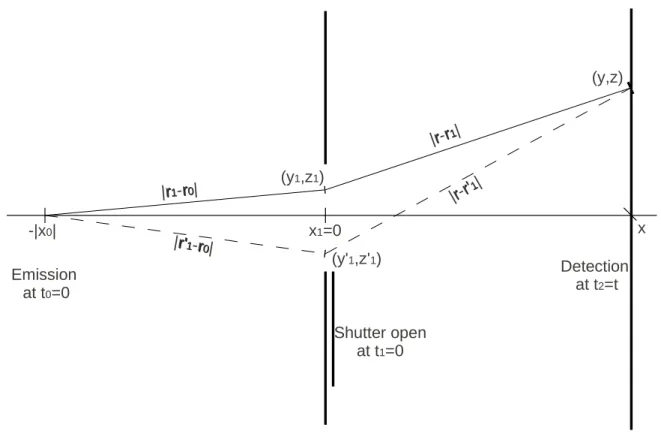
(42) and whereρ≡ |r−r₁|+|r₁−r₀|can be interpreted as the semi-classical path length traveled by the particle: see Fig. 1. Hence the one-slit propagator formula (28) can be written as follows:

K_sc^(a,b)(r, t;r₀,0) = e^imx2~t2 (2iπ~t/m)^1/2

Z a

−a

dz1

Z b

−b

dy1 σt,τsc(x, x0)e^{im[(y−y2~1)(t−τsc)2+(z−z1)2]}

2iπ~(t−τ_sc)/m e^im[y

21 +z2 2~τsc1]

2iπ~τ_sc/m (43) The formula (43) is similar to the one-point source propagator in the truncation approx- imation, formula (85) of Appendix 1, except that the semiclassical time τsc depends on the distance from the origin to the point in the slit, and from the slit to the screen (see (37)), and the functionσt,τsc in front of the product of the two Gaussians depends on the boundary conditions.

Remark 1. We can give a geometric interpretation to the diffraction in space and in time in the semiclassical regime. The first-order term of the semiclassical approximation (41) gives only the classical path contribution. Therefore, we observe that the propagator (43) is nothing but a sum over allsemiclassical paths (made up of two broken lines) passing through

FIG. 1. Schematic representation of the apparatus. We illustrate two interfering classical paths starting fromr₀ at the timet₀ = 0 torat the timetand passing through the aperture at r₁ (resp.

r^′₁) at the timeτsc (resp. τ_sc^′ ) given by the formula (37).

the aperture of the slit as in Fig.1. Thus, the equation (43) shows that the semiclassical approximation is in fact a truncation approximation since one sees in these formulas that the motion along thex-axis and the motion in the orthogonal (y, z) plane are separated and moreover that along the x-axis the motion is classical. However, we have more information within our model since by (37) we notice that there is a relation between the classical times τsc and t even if the two motions from the source to the slit and from the slit to the screen are separated, see Fig. 1. Actually, we can interpret this relation as the conservation of the

classical energy of the particle when the particle passes through the slit:

E(r1, τsc) =E(r, t)⇔ m 2

r₁−r₀ τsc−t0

2

= m 2

r−r₁ t−τsc

2

and this leads to (37), whereas the classical momentum is not conserved due to the quantum diffraction phenomenon.

Consequently, in the semiclassical regime, the theory of diffraction in time allows us to take into account all the classical paths (passing through the slit at a time depending on the position inside the aperture) without assuming that the dimensions of the aperture are small compared to the dimension of the apparatus along thex-axis. Moreover, the additional term (42) which could not be discovered otherwise, has an important physical meaning since the values of the parameters η1, η2 depend on whether the screen of the slit is reflective, absorbing or neither.

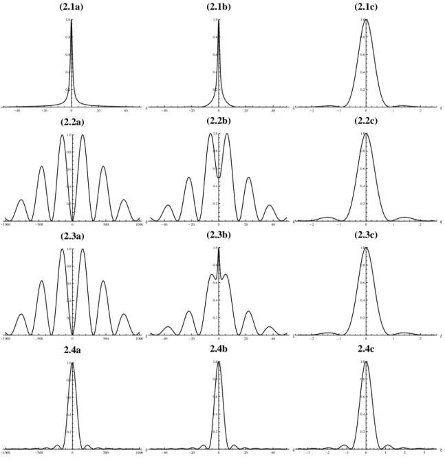
In Fig.2., Appendix 3 we show the transition between the quantum and the semiclassical regimes from the left to the right.

Firstly, for the diffraction patterns at the left side (Fig.2.1a-2.4a), the semiclassical pa- rameter µ∼4 (i.e., relatively close to one) and so that explain why the curves are different from those for the truncation approximation (see Fig.2.4a). We observe that for the Dirich- let boundary condition (Fig.2.1a) there is a narrow central peak decreasing very fast so that we can not see the oscillations (a numerical zoom could show these slight oscillations). On the contrary, for the Neumann (Fig.2.2a) and the free boundary conditions (Fig.2.3a), there is no central peak but large oscillations where the distance between the fringes is essentially constant but different from the distance between the fringes in the truncation approximation (Fig.2.4a).

For the curves at right side of (Fig.2.1c-2.4c), we have µ ∼ 800 ≫ 1 and then we get similar pictures to those in the truncation approximation (Fig. 2.4c) although there is still a difference in the location of the fringes. In the following section, we will give a qualitative description of those differences. From (72) and (76) we can conclude that if the first minima of the curves are not too different, however we observed that the second and the third differ by 50%.

The patterns in the middle of Fig.2, show the transition between the quantum and the semiclassical regimes where a central peak appears also for the Neumann (Fig.2.5) and the free boundary conditions (Fig.2.8).

Remark 2. Let us make another remark about the probabilistic interpretation of the slit diffraction experiment in the semiclassical limit. A consequence of the last comment about the relation between the semiclassical approximation and the truncation approximation is that there is an analogous equation to (26) giving the relation of the conservation of the probability between the aperture of the slit and the screen:

Z b

−b

dy1

Z a

−a

dz1 |ψsc(r1, τsc)|² = Z +∞

−∞

dy Z +∞

−∞

dz |ψsc(r, t)|² ≡Msc (44) where τsc is given by (37) and depends on r,r₁,r₀, t, and where the semiclassical wave functions in (44) are given by:

ψsc(r₁, τsc) = Z

R³

dR G0(r₁−R, τsc) e^i|

R−r0|2 2σ2

(2πσ²)^3/2 (45)

ψsc(r, t) = Z

R³

dR K_sc^(a,b)(r, t,R,0) e^i|

R−r0|2 2σ2

(2πσ²)^3/2 (46)

So we get the following formula for the semiclassical density of probability:

Psc(r, t) = 1

Msc|ψsc(r, t)|² → 1

Ωsc|K_sc^(a,b)(r, t,r₀,0)|², when σ →0 (47) where Msc is defined in (44) and Ωsc =Rb

−bdy1

Ra

−adz1 |G0(r1−R, τsc)|².

IV. SEMI-CLASSICAL APPROXIMATIONS FOR THE SLIT EXPERIMENT

The equation (28) gives the three-dimensional one-gate-slit propagator as a double in- tegral of the three-dimensional one-point-slit propagator given by the equations (30), (32) and (31). Despite the fact that there is no explicit formula giving the result for the gate-slit propagator, we can give an approximation when the size of the slit and the distance on the screen are relatively small, in which case it is also of interest to give an estimate for the relative shift between the minima in the interference pattern for the Fraunhofer regime compared with the truncation approximation.

We first want to give the semiclassical approximation of the one-point source propagator (30) when the sizes in the x-direction are relatively large compared to the sizes of the slit and of the distances of the observation point on the screen:

|x−x1|,|x1−x0| ≫a, b,|z|,|y|

and also large compared to λ₀ =p

2π~t/m (relatively short time). Therefore the semiclas- sical limit (43) is a good approximation.

By (31), the phase of the propagator (30) is given by

~

mϕt = |r−r₁|²

2t + |r₁−r₀|²

2t + |r−r₁||r₁−r₀|

t (48)

We denote the two-dimensional vectors of the position on the screen r_⊥ = (y, z), on the slit r_⊥,1 = (y1, z1). In the sequel, we take x1 = 0, so |x−x1| = |x|, |x1 −x0| = |x0| and y0 = 0, z0 = 0, x0 <0. The first two terms of the r.h.s. of (48) are rewritten as

|r−r₁|²

2t +|r₁|² 2t = x²

2t +(r⊥−r_⊥,1)² 2t + x²₀

2t +r²_⊥,1

2t (49)

Expanding to fourth order the third term of the r.h.s. of (48), we have

|r−r₁||r₁−r₀|

t = |x||x0| t

r

1 + (r⊥−r_⊥,1)² x²

s

1 + r²_⊥,1

x²₀ (50)

≈ |x||x0| t

1 + (r⊥−r_⊥,1)²

2x² − (r⊥−r_⊥,1)⁴

8x⁴ 1 + r²_⊥,1

2x²₀ − r⁴_⊥,1 8x⁴₀

(51)

≈ |x||x0| t

1 + r²_⊥,1

2x²₀ +(r⊥−r_⊥,1)² 2x²

−|x||x0| 8t

(r⊥−r_⊥,1)²

x² − r²_⊥,1 x²₀

²

(52) Due to (49) and (52) we get:

~

mϕt ≈ (x−x0)²

2t +(r_⊥−r_⊥,1)²

2(t−tc) + r²_⊥,1

2tc − |x||x0| 8t

(r_⊥−r_⊥,1)²

x² − r²_⊥,1 x⁴₀

²

(53) where:

t_c = |x₀|

|x|+|x0|t= |x₀|

|x−x0|t . (54)

A. The truncation approximation

Notice that due to (37),tc could be interpreted as the semiclassical time at the first order approximation in the regime |x|,|x₀| ≫ |z|,|z₁|:

τsc = |r₁−r₀|t

|r−r₁|+|r₁−r₀| ≈tc, when |x|,|x0| ≫ |z|,|z1| . (55) Inserting this into the amplitude of (41), i.e. neglecting the influence of the position on the screen and in the slit, we get the following approximation:

At(r,r₀|r₁)≈σt,tc(x, x0) 1 p2iπ~t/m

1

(2iπ~/m)²(t−tc)tc

. (56)

whereσt,tc(x, x0) is given by (42). In (53), we neglect the terms of order O(r⁴_⊥) andO(r⁴_⊥,1), to get

~

mϕt≈ (x−x0)²

2t + (r⊥−r_⊥,1)²

2(t−tc) +r²_⊥,1 2tc

. (57)

Then, by (56) and (57), we get the Fraunhofer approximation to second order for the one- point source propagator:

Kt(r,r₀|r₁)≈ σ_t,tc(x, x₀) e^im(x−x0)

2 2~t

p2iπ~t/m

e^im(y−y1)

2 2~(t−tc)

p2iπ~(t−tc)/m

e^{im y}

12 2~tc

p2iπ~tc/m

e^im(z−z1)

2 2~(t−tc)

p2iπ~(t−tc)/m

e^{im z}

21 2~tc

p2iπ~tc/m . (58) Consequently, for the single-slit model, by integrating over y1, z1 on [−b, b]×[−a, a], we get the usual truncation approximation formula (86), see Appendix 1, multiplied by a constant factor σt,tc depending on t and tc, as well as on |x0|, x and on the boundary conditions.

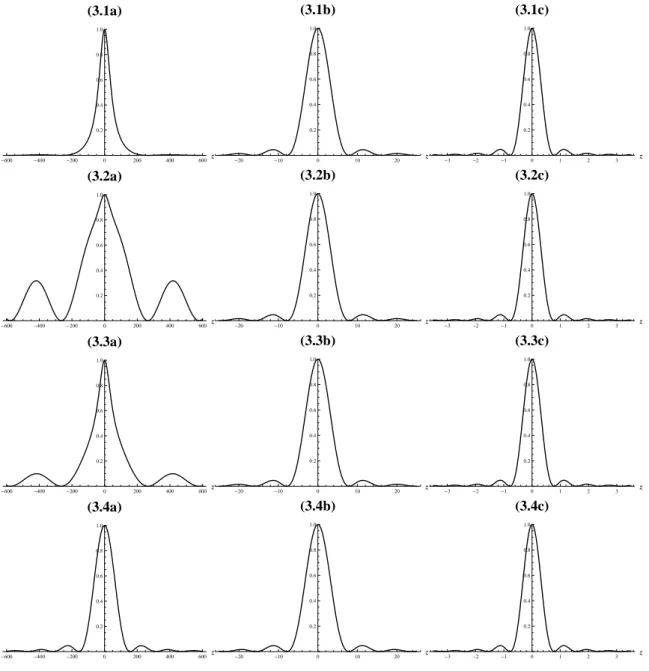
In addition, by the semiclassical probabilistic interpretation, see (47), since σ_t,tc(x, x₀) is a constant number, we get the same probability density formula as the one in¹⁴, (see also (96) in Appendix 1) which means that the initial boundary conditions on the slit do not affect the diffraction pattern in this regime. We observe this phenomenon numerically in Fig.3.

for t= 0.05 and t= 0.005.

B. The fourth-order approximation in the Fraunhofer regime

Remember that the Fresnel numbers (see Appendix 1) are given by NF(a) = 2a²

λL, NF(b) = 2b² λL

where L = |x| and λ = 2π~/(mv), and where a is the dimension of the slit along the z- axis and b the one along the y-axis, with v ≈ vx = |x−x0|/t. In the Fraunhofer regime, we have NF(a) ≪ 1 and since the distance between two successive minima on the pattern is ∆z ∼ λL/(2a) = a/Nf(a) (see Fig. 3 for the truncation model (TM) and¹⁴), we have

∆z ≫a and so we are looking for the correction forz ≫a. We also assume that x≫b≫a and 2b²/(λL) ≪ 1, so that ∆z ≫ ∆y ≫ b. In this case, we can neglect the terms of the order O(y⁴) and O(y₁⁴) in (53):

~

mϕt ≈ x²

2t + (r⊥−r_⊥,1)²

2(t−t_c) +r²_⊥,1

2t_c −|x||x0| 8t

(z−z1)² x² − z₁²

x²₀ 2

(59)