HAL Id: hal-00466861
https://hal.archives-ouvertes.fr/hal-00466861
Submitted on 25 Mar 2010
HAL is a multi-disciplinary open access archive for the deposit and dissemination of sci- entific research documents, whether they are pub- lished or not. The documents may come from teaching and research institutions in France or
L’archive ouverte pluridisciplinaire HAL, est destinée au dépôt et à la diffusion de documents scientifiques de niveau recherche, publiés ou non, émanant des établissements d’enseignement et de recherche français ou étrangers, des laboratoires
Résumé de Séquences Temporelles pour le passage à l’échelle d’applications dépendantes du temps
Quang-Khai Pham, Guillaume Raschia, Régis Saint-Paul, Boualem Benatallah, Noureddine Mouaddib
To cite this version:
Quang-Khai Pham, Guillaume Raschia, Régis Saint-Paul, Boualem Benatallah, Noureddine Mouaddib.
Résumé de Séquences Temporelles pour le passage à l’échelle d’applications dépendantes du temps.
25èmes journées Bases de Données Avancées (BDA), Oct 2009, Namur, Belgium. Article accepté n°9.
�hal-00466861�
R´esum´e de S´equences Temporelles pour le Passage `a l’ ´ Echelle d’Applications D´ependantes du Temps
Quang-Khai Pham
†‡, Guillaume Raschia
‡, Regis Saint-Paul
⋆, Boualem Benatallah
†, Noureddine Mouaddib
‡‡
LINA CNRS UMR 6241 - Atlas group University of Nantes, France
{noureddine.mouaddib, guillaume.raschia}@univ-nantes.fr
⋆
CREATE-NET Trento 38100, Italy
regis.saint-paul@create-net.org
†
CSE at UNSW
Sydney, NSW 2033, Australia {qpham, boualem}@cse.unsw.edu.au
Abstract
Nous pr´esentons dans ces travaux le concept du “R´esum´e de S´equence Temporelle” dont le but est d’aider les applications d´ependantes du temps `a passer `a l’´echelle sur de grandes masses de donn´ees.
Un R´esum´e de S´equence Temporelle s’obtient en transformant une s´equence d’´ev´enements o`u les ´ev´ene- ments sont ordonn´es chronologiquement. Chaque ´ev´enement est pr´ecis´ement d´ecrit par un ensemble de labels. Le r´esum´e produit est alors une s´equence temporelle d’´ev´enements, plus concise que la s´equence originale et pouvant se substituer `a l’originale dans les applications. Nous proposons un algorithme ap- pel´e “TSaR” pour produire un tel r´esum´e. TSaR se base sur les principes de g´en´eralisation, de regroupe- ment et de formation de concept. La g´en´eralisation permet d’abstraire `a l’aide de taxonomies les labels qui d´ecrivent les ´ev´enements. Le regroupement permet ensuite d’agglom´erer les ´ev´enements g´en´eralis´es qui sont similaires. La formation de concept r´eduit le nombre d’´ev´enements group´es-g´en´eralis´es dans la s´equence en repr´esentant chaque groupe form´e par un unique ´ev´enement. Le processus est conc¸u de mani`ere `a pr´eserver la chronologie globale de la s´equence d’entr´ee. L’algorithme TSaR produit le r´esum´e de mani`ere incr´ementale et a une complexit´e algorithmique lin´eaire. Nous validons notre approche par un ensemble d’exp´eriences sur une ann´ee d’actualit´es financi`eres produites par Reuters.
Keywoards: Time sequences, Summarization, Taxonomies, Clustering
1 Introduction
Domains such as medicine, the WWW, business or finance generate and store on a daily basis mas- sive amounts of data. This data is represented as a collection of time sequences of events where each
event is described as a set of descriptors taken from various descriptive domains and associated with a timestamp. These archives represent valuable sources of insight for analysts to browse, analyze and discover golden nuggets of knowledge. For instance, biologists could discover disease risk factors by analyzing patient history [28], web content producers and marketing people are interested in profiling client behaviors [24], traders investigate financial data for understanding global trends or anticipating market moves [30]. However, analysts are overloaded with the size of this data and increasingly need methods and tools allowing exploratory visualization, query or analysis.
As an example, Google has developed Google Finance [1]. In a user-defined timeline, Google Finance provides analysts with a tool to browse through companies’ stock values while visualizing background information about the companies. This background information is provided in the form of a sequence of chronologically ordered news events that appeared at some interesting moments, e.g., during price jumps. We call applications, such as Google Finance, that rely on the chronological order of the data to be meaningful: Chronology-dependent applications.
In this context, we observed that sequences of events relating to an entity A occurring in a short period of time are likely to relate to a same topic, e.g., events about Lehman Brothers mid-September 2008 relate to its bankruptcy. This observation shows that it could be more practical and meaningful for the analyst to navigate in the chronology of events through summarized events that gather several events about a same topic, e.g., Lehman Brothers’s Backruptcy, rather than the entire set of individual events. At the same time, the analyst should be given the possibility to browse the details of these summarized events for a more in-depth analysis. This existing example puts forward the need for a data representation where multiple events describing a same topic are grouped while preserving the overall chronology of events’ topic.
During the past decade, semantic data summarization has been addressed in various areas such as databases, data warehouses, datastreams, etc., to represent data in a more concise form by using its semantics [10, 11, 14, 5, 13, 23]. However, including the time dimension into the summarization process is an additional constraint that requires the chronology of events’ topic to somehow be preserved. For instance, the sequencehLehman Brothers’s Bankruptcy, Lehman Brothers’s Rescuei only makes sense because the events related to the Bankruptcy need to occur before the Rescue can happen. We name this type of data transformation, based on the data’s semantic content and temporal characteristics, Time Sequence Summarization. A time sequence summarizer should take as input a time sequence of events, where each event is described by a set of descriptors, and output a time sequence of summarized events.
The produced summarized time sequence should have the following properties:
1. Brevity: The number of summarized events in the output time sequence should be reduced in comparison to the number of events in the input time sequence.
2. Substitution principle: A chronology-dependent application that performs on a time sequence of events should be capable of performing seamlessly if the input time sequence is replaced by its summary.
3. Informativeness: Summarization should reduce time sequen- ces of events in a way that keeps the semantic content available to and understandable by the analyst without the need for desummarization.
4. Accuracy and usefulness: The input time sequence of events should not be overgeneralized to preserve descriptive precision and keep the summarized time sequence useful. However, ensuring high descriptive precision of events in the summarized time sequence requires trading off the brevity property of the summary.
5. Chronology preservation: The chronology of summarized events in the output time sequence should reflect the overall chrono- logy of events in the input time sequence.
6. Computational scalability: Time sequence summaries are built to support chronology-dependent applications and, thus their construction should not become a bottleneck. Applications such as data mining might need to handle very large and long collections of time sequences of events, e.g., news feeds, web logs or market data, to rapidly discover knowledge. Therefore, the summarization process should have low processing and memory requirements.
Designing a time sequence summary that displays all these properties is a challenging task. There ex- ists a bulk of work for designing summaries in different areas such as datastreams, transaction databases, event sequences or relational databases. However, to the best of our knowledge, this research corpus does not address simultaneously all six mentioned properties.
Contributions. In this paper, we present the concept of Time Sequence Summarization and propose a summarization technique that satisfies all six mentioned properties to support chronology-dependent applications. Our contributions are as follows:
• We give a formal definition of Time Sequence Summarization. The time sequence summary of a time sequence of events is a time sequence of summarized events where: (i) events occurring close in time and relating to a same topic are gathered into a same summarized event and (ii) each summarized event is represented by a concept formed from the underlying events. For example, assume the input time sequence of events is: h(t1,Easy subprime loan),(t2,Interest rate increase),(t3,Housing market collapse)i. A valid time sequence summary could be: h(t′1,Subprime crisis)i.
•We propose a Time Sequence SummaRization (TSaR) algorithm. TSaR relies on the ideas of Gen- eralization and Merging, introduced by Han et al. for discovering knowledge in relational databases [10, 11]. TSaR is a 3-step process that uses background knowledge in the form of taxonomies, supposedly given by the analyst to generalize event descriptors at higher levels of abstraction.
Assuming events occurring close in time might relate to a same topic, grouping is performed on gen- eralized events whose generalized descriptors are similar. TSaR’s grouping process gathers generalized events in a way that respects the chronology of topics in the input time sequence. For this purpose, a Temporal Locality is defined so that temporally close events can be gathered. Temporal locality is a term borrowed from Operating systems research [8] and defined in Section 4.3. It can intuitively be under- stood as the fact that a series of events close in time have high probability of relating to a same topic.
However, events relating to different topics might locally overlap in that period, e.g., due to network delays. Thus, defining a temporal locality allows TSaR to gather these overlapping events into their cor- responding topics. Finally, each group is represented by a concept. In total, higher numerosity reduction can be achieved while the chronology of topics in the input time sequence is preserved.
TSaR summaries are built in an incremental way by processing an input time sequence of events in a one-pass manner. The algorithm has small memory and processing footprints. TSaR maintains in- memory a small structure that holds a limited number of grouped events, i.e., grouped events that fit into the temporal locality. TSaR’s algorithmic complexity is linear with the number of events in the input time sequence.
We validate these characteristics with a set of experiments on real world data. We performed experi- ments using one year of English financial news events obtained from Reuters’s. These archives contain after cleaning and preprocessing approximately 1.28M events split over 34458 time sequences. Each event in the time sequences is a set of words that precisely describes the content of the corresponding
news article. Our extensive set of experiments on summarizing this data shows that TSaR has (i) inter- esting numerosity reduction capabilities, e.g., compression ratio ranges from 10% to 82%, and (ii) low and linear processing cost.
Roadmap. The rest of the paper is organized as follows. Section 2 presents related work. Section 3 formalizes the concept of Time Sequence Summarization. Section 4 presents the novel technique we contribute in the paper. Section 5 discusses the experimentation we performed on financial news data.
We conclude and discuss future work in Section 6.
2 Related work
Our work relates to lines of research, where a concise representation of massive data sources is de- sirable for storage or for knowledge discovery in constrained processing and memory environments.
Related research domains are those where summaries are built from sequences of objects ordered by their time of occurrence. In this context, and in the light of the requirements mentioned in the introduc- tion, we examine summarization techniques produced for datastreams, transaction databases and event sequen- ces. This study, however, do not encompass time series summarization as time series summa- rization rely on methods that only consider numerical data.
Datastreams. Datastreams is a domain characterized by data of infinite size and eventually generated at very high rates. The common assumptions are that (i) any processing should be performed in a sin- gle pass and (ii) input data can not be integrally stored. Such constraints have motivated researchers to represent input streams in a more concise form to support analysis applications, e.g., (approximate) con- tinuous queries answering, frequent items counting, aggregation, clustering, etc.. Techniques proposed maintain in memory small structures, e.g., samples, histograms, quantiles or synopses, for streams of numerical data (we refer the reader to [9] for a more complete review). In contrast with numerical data that is defined on continuous and totally ordered domains, categorical descriptors are defined on discrete and partially ordered domains. Therefore, descriptors can not be handled and reduced in the same way as numerical data using conventional datastreaming summarization techniques, e.g, min/max/average functions.
To the best of our knowledge, small interest has been given to designing summaries[4, 23] for cate- gorical datastreams. Aggarwal et al. [4] proposed a clustering method for categorical datastreams. The approach relies on the idea of co-occurrence of attribute values to build statistical summaries and gather input data based on these statistics. However, the clusters built do not reflect the chronology of the input data and require pre-processing before analysis. We proposed in previous work an approach to summarize datastreams using a conceptual summarization algorithm [20]. The summary produced does not reflect the chronology of the input data and can not be directly exploited by chronology-dependent applications.
Transaction database summarization. Transaction databases (TDB) are collections of time se- quences where each time sequence is a list of chronologically ordered itemsets. A bulk of work [6, 25, 26, 29] has focused on creating summaries for transaction databases. Chandola et al.’s approach [6] and SUMMARY [26] are techniques that rely on closed frequent itemset mining to build an informative rep- resentation that covers the entire TDB. Building these summaries require multiple passes over the input TDB and the output is a set of frequent itemsets. This output does not endorse the substitution principal and does not reflect the chronology of transactions of the input TDB. HYPER [29] summarizes a TDB
as a set of hyperrectangles that covers the database. HYPER’s output set of hyperrectangles requires preprocessing before chronology-dependent applications can exploit the summary and hyperrectangles are computed in polynomial time. But, designing a time sequence summarizer requires a single pass over the data and the output to preserve the chronology of transactions. Wan et al. [25] summarize a TDB into the compact form of a CT-tree specifically to support Sequential Pattern Mining (SPM). The output tree structure allows SPM to perform but looses the chronology of transactions of the input TDB.
Event sequence summarization. Kiernan and Terzi [16] rely on the Minimum Description Length (MDL) principle to produce in a parameter-free way a comprehensive summary of an event sequence, where events are taken from setE ofm different event types. The authors segment the input event se- quence timeline intoksegments. Summarization is achieved by describing each segmentSi with a local modelMithat is a partition ofE where groupsXij ∈Migather event types of similar rate of appearance inSi. Each event groupXij ∈Miis then associated with a probability of appearancep(Xij)ofXij inSi. However, the output summary can not be directly piped to a chronology-dependent application and needs some form of desummarization. Hence, the authors’ definition of summarization does not endorse the substitution principle and one can not seamlessly substitute the original event sequence for the summary.
The TSaR approach builds on top of the ideas in Attribute Oriented Induction (AOI) [10, 11]. The TSaR process is split into three sub-routines that allow input time sequences to be processed in an incre- mental way: (i) generalization, (ii) grouping and (iii) concept formation. Generalization transforms event descriptors into a more abstract but informative form. Then, grouping gathers generalized events that are semantically close, i.e., having similar generalized descriptors, and chronologically close. Grouping is performed in a way that preserves the overall chronology of topics in the time sequence. Finally, each formed group is represented by a concept, i.e., a set of descriptors, formed from the underlying events’ descriptors. The output can then be directly interpreted by a human analyst or piped to any chronology-dependent application.
3 Time sequence summary
In this section, we give a running toy example to illustrate all the concepts presented in this paper.
We also introduce the basic terminology used throughout the rest of the discussion and formalize the concept of Time Sequence Summarization.
3.1 Toy example
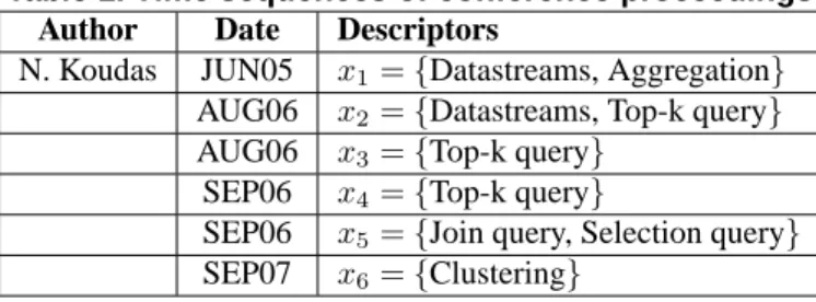
To illustrate the ideas exposed in this paper, we generate in Table 1 a simple toy example with a time sequence extracted from conference proceedings. The author N. Koudas is associated with a time sequence where each event is one publication timestamped by its date of presentation. For simplicity, the set of descriptors describing an event is taken from one single descriptive domain, namely, the paper’s topic. Without loss of generality, this discussion is valid for any number of descriptive domains. This example is purposely unrelated to the application domain we provide in Section 5. It illustrates all the concepts introduced and shows the genericity of our approach.
Table 1. Time sequences of conference proceedings Author Date Descriptors
N. Koudas JUN05 x1={Datastreams, Aggregation}
AUG06 x2={Datastreams, Top-k query}
AUG06 x3={Top-k query}
SEP06 x4={Top-k query}
SEP06 x5={Join query, Selection query}
SEP07 x6={Clustering}
3.2 Terminology
LetΩbe the universe of discourse, i.e., the set of all descriptors that could describe an event in a time sequence of events. Ω = S
ADA is organized into several descriptive domains DA corresponding to each domainAthat interests the analyst, e.g., the topic of research papers.
We refer to a part ofΩ, i.e., a subset of descriptors taken from various descriptive domains, asP(Ω).
An itemsetxis defined as an element inP(Ω). Given an object of interest (e.g., “N. Koudas”), an event e is defined by an itemsetxthat describese(e.g.,{Datastreams, Aggregation}) and is associated with a timestampt(e.g.,t=“JUN05”). We assume the data input for time sequence summarization, also called raw data, is a collection of time sequences of events as defined in Definition 1.
Definition 1 (Time Sequence of events)
A time sequence of eventss=h(x1, t1), . . . ,(xm, tm)i, also called time sequence for short, is a series of events(xj, tj), with1≤j ≤mandxj ∈ P(Ω), ordered by increasing timestamptj. We denote byS = {x1, . . . , xm}the support multi-set ofs. A time sequencesverifies: ∀(xj, xk)∈ S2, j < k ⇔tj < tk. We denote bys[T]the set of timestamps of elements inS.
This definition of a time sequence and the total order on timestamps allow us to equivalently write:
s=h(x1, t1), . . . ,(xm, tm)i ⇔s={(xj, tj)},1≤j ≤m
By convention, we further simplify the notation of a time sequence and notes=hx1, . . . , xmiwhere eachxj,1≤j ≤m, is an itemset and all itemsetsxj are sorted by ascending indexj. This simplification of the notation allows us to interchangeably use the term event to refer to the itemsetxj in event(xj, tj).
We denote byS(Ω)the set of time sequences inP(Ω). This notion of time sequence can be generalized and used to define a sequence of time sequences that we hereafter call second-order time sequence.
Second-order time sequences are more formally defined in Definition 2.
Definition 2 (Second-order time sequence)
A second-order time sequence defined onΩis a time sequence s = {(yi, t′i)}where each event(yi, t′i) is itself a regular time sequence of events defined onΩ. Events(yi, t′i)ins, where yi = {(xj, tj)}, are ordered thanks to the minimum timestamp value t′i = min{tj}. The set of second-order time sequences defined onΩis denotedS2(Ω).
An example of second-order time sequence from Table 1 for author N. Koudas can be defined as fol- lows: s=h(y1, t′1),(y2, t′2),(y3, t′3))iwhere:
•y1=h(x1={Datastreams, Aggregation},t1=JUN05)iandt′1=t1=JUN05
•y2=h(x2, t2),(x3, t3),(x4, t4),(x5, t5))iandt′2 =min{t2, . . . , t5}i.e.,t′2=AUG06, where:
−x2={Datastreams, Top-k query}andt2=AUG06
−x3={Top-k query}andt3=AUG06
−x4={Top-k query}andt4=SEP06
−x5={Join query, Selection query}andt5=SEP06
•y3=h(x6={Clustering},t6=SEP07)iandt′3=t6=SEP07
A second-order time sequence can be obtained from a time sequences as defined in Definition 1 by the means of a form of clustering based on the semantics and temporal information of events xi,j ins.
We refer the reader to the following surveys for more indepth on clustering [15, 27]. Reversely, a time sequence can be obtained from a second-order time sequencesby means of concept formation [18, 19]
computed from time sequencesyiins.
3.3 Time sequence summary
We formally define in Definition 3 the concept of a time sequence summary using the concepts intro- duced previously.
Definition 3 (Time sequence summary)
Given a time sequences={(xi, ti)} ∈ S(Ω), using clustering terminology, we define the time sequence summary ofs, denotedχ(s) = (s2C, s⋆M)∈ S2(Ω)× S(Ω), as follows:
• s2C ={(yi, t′i)}is a second-order time sequence where eventsyi ∈s2C are clusters obtained thanks to a form of clusteringCthat relies on events(xi, ti)semantic and temporal information.
• s⋆M ={(x⋆i, t′i)}is the time sequence of conceptsx⋆i formed from clustersyi ∈s2C. M is the model chosen to characterize each clusteryi ∈s2C, i.e., to build the concepts.
Hence,s2C ands⋆M can be understood as the extension and the intention, respectively, of summaryχ(s).
We defined time sequence summarization using clustering terminology as the underlying ideas are similar, i.e., grouping objects based on their proximity. The novelty of time sequence summaries relies on the fact that events are clustered thanks to their semantic and temporal information. Conventional clustering methods mostly rely on the joint features of the objects considered and their proximity is evaluated thanks to a distance measure, e.g., based on entropy or semantic distances. Similarly, in time sequence summarization, a form of temporal approximation should also be applicable so that objects that are close from temporal view point are grouped. Consequently, local rearrangement of the objects on the timeline should also be allowed.
In a nutshell, the objective of time sequence summarization is to find the best method for grouping events based on their semantic content and their proximity on the timeline. This general definition of time sequence summarization can partially encompass some previous works such as Kiernan and Terzi’s research on large event sequences summarization [16]. Indeed, the authors perform summarization by partitioning an event sequenceS intoksegmentsSi,1≤i≤k; this segmentation can be understood as organizingSinto a second-order time sequences2C whereCis their segmentation method, e.g., Segment- DP. Note that the authors’ segmentation method does not allow any form of event rearrangement on the timeline. Then, each segmentSiis described by a set of event type groups{Xi,j}where eachXi,jgroups event types of similar appearance rate. Thus, the model used to describe each segment is a probabilistic model. To this point, our definition of a time sequence summary fully generalizes Kiernan and Terzi’s
work. However, the authors add for eachXi,j its probability of appearancep(Xi,j)inSi. By doing so, the authors do not support the substitution principle and thus do not completely respect our definition of a time sequence summary.
4 The TS
AR approach
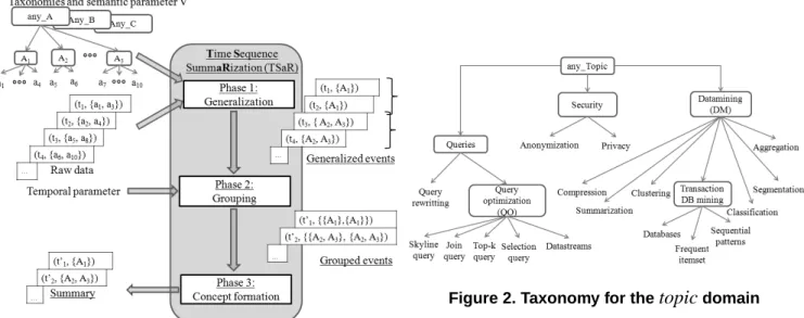
In this section we present a Time Sequence SummaRization technique called TSaR. The basic princi- ple of TSaR is illustrated in Figure 1. The idea is to gather events whose descriptors are similar at some high level of abstraction and that appear close in time. This is done in three steps: (i) reduce the data’s domain of representation by generalizing descriptors to a user defined level of abstraction, (ii) group identical sets of descriptors within a certain sliding time window then (iii) represent each group with a single set of descriptors, a.k.a. concept.
In practice, the process is parametrized by three inputs: (i) domain specific taxonomies, (ii) a semantic accuracy parameter and (iii) a temporal precision parameter. The generalization process in phase 1 takes as input a time sequence, domain specific taxonomies and the user defined semantic accuracy parameter.
It outputs a time sequence of generalized events where event descriptors are expressed at higher levels of taxonomy. This output is then fed to the grouping process in phase 2 where identical generalized events are grouped together. The overall chronology of events is preserved by grouping only generalized events present in a same temporal locality (as defined in Section 4.3). Phase 3 forms a concept to represent each group. Here, since all sets of descriptors in a group are identical, one instance of the group is selected to represent the group. We will detail these steps in the following sections.
Figure 1. TSaR summarization process
Figure 2. Taxonomy for thetopicdomain
4.1 Preliminaries
In this work, we assume that each descriptive domainDA, on which event descriptors are defined, is structured into a taxonomyHAthat defines a generalization-specialization relationship between descrip- tors ofDA. The set of all taxonomies is denoted H = S
AHA. The taxonomy HA provides a partial
ordering≺Aover DAand is rooted by the special descriptorany A, i.e.,∀a ∈ DA, a ≺A any A. For convenience, we assume in the following that the descriptorany Abelongs toDA.
The partial ordering≺A onDA defines a cover relation <A that corresponds to direct links between items in the taxonomy. Hence, we have∀(x, y) ∈ D2A, x ≺A y ⇒ ∃(y1, y2, . . . , yk) ∈ DAk such that x <Ay1 <A. . . <Ayk <A y. The length of the path fromxtoyisℓ(x, y) =k+ 1. In other words, we needk+ 1generalizations to reachyfromxinHA. For example, given the topic taxonomy in Figure 2, it takes 2 generalizations to reach the concept Queries from the concept Top-k query.
In practice, we assume these taxonomies are available to the analyst. We believe this assumption is realistic as there exists numerous domain specific ontologies available, e.g., WordNet [3] or Onto-Med for medicine, as well as techniques that allow the automatic generation of taxonomies [17, 22].
4.2 Generalization phase
Here, we detail the generalization phase that uses taxonomies to represent the input data at higher levels of abstraction. We assumed values inΩare partially ordered by the partial order relation≺A, so, thanks to this relation, we can define a containment relation⊑over subsets ofΩ, i.e.,P(Ω).
∀(x, y)∈ P(Ω)2, (x⊑y) ⇐⇒ ∀i∈x, ∃i′ ∈y, ∃A∈ A, (i≺A i′)∨(i=i′)
For generalization, we need to replace event descriptors with upper terms of the taxonomies. We call generalization vector onΩ, denotedϑ ∈ Ni, a list of integer values. ϑ defines the number of general- izations to perform for each descriptive domain inA. We denote byϑ[A]the generalization level for the domainA. Equipped with this generalization vectorϑ, we are now able to define a restriction⊑↓ϑ of the containment relation above:
∀(x, y)∈ P(Ω)2, (x⊑↓ϑy)⇐⇒
∀i∈x,∃i′ ∈y,∃A∈ A, (i≺Ai′)∧ (ℓ(i, i′) =ϑ[A])∨((ℓ(i, i′)< ϑ[A])∧(i′ =any A))
Definition 4 (Generalization of a Time Sequence)
Given a generalization vector ϑ and a set of taxonomies H, we define a parametric generalization functionϕϑthat operates on a time sequences=hx1, . . . , xnias follows:
ϕϑ: S(Ω) −→ S(Ω)
s 7−→ ϕϑ(s) =hx′1, . . . , x′nisuch that∀i∈ {1..n}, xi ⊑↓ϑ x′i
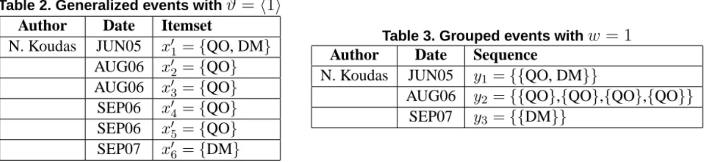
For example, given the topic taxonomy in Figure 2 the generalized version of Table 1 with a general- ization vectorϑ[topic] = 1(also denotedϑ = h1iwhen all taxonomies should be generalized once) is shown in Table 2. We can notice that the⊑↓ϑrelation also allows to reduce itemsets’ cardinality. Indeed, Datastreams and Top-k query both generalize into QO. As a result, in N. Koudas’s time sequence, the event{Datastreams, Top-k query}is generalized into{QO}.
From the analyst’s view point, ϑ represents the semantic accuracy he desires for each descriptive domain. If he is interested in the minute details of a specific domain, e.g., a paper’s topic, he can set ϑ to a low value, e.g., ϑ[topic] = 0 or ϑ[topic] = 1. Otherwise, he can set ϑ to higher values for a more abstract description of the domain. Once the input time sequence has undergone generalization, the output undergoes a grouping process as described in the following section.
Table 2. Generalized events withϑ=h1i Author Date Itemset
N. Koudas JUN05 x′1={QO, DM}
AUG06 x′2={QO}
AUG06 x′3={QO}
SEP06 x′4={QO}
SEP06 x′5={QO}
SEP07 x′6={DM}
Table 3. Grouped events withw= 1 Author Date Sequence
N. Koudas JUN05 y1={{QO, DM}}
AUG06 y2={{QO},{QO},{QO},{QO}}
SEP07 y3={{DM}}
4.3 Grouping phase
Here, we detail the grouping phase responsible for gathering generalized events. This phase relies on two concepts: (i) second-order time sequence as defined in Definition 2 and (ii) Temporal locality. We define this notion of temporal locality hereafter.
4.3.1 Temporal locality
In many research areas, it is assumed that a sequence of events generated close in time have high probability of relating to a same topic. This notion of temporal locality is borrowed from Operating systems research [8]. For example, hPaper deadline, Authors notification, Camera-ready paperi is a chronology of events describing the Conference submission topic. However, in a time sequence, events describing different topics can eventually be intertwined, e.g., due to network delays. Thus, defining a temporal locality for grouping events of a time sequence allows to capture the following notions: (i) sequentiality of events for a given topic and (ii) chronology between topics.
Temporal locality is measured as the time differencedT, on a temporal scaleT, between an incoming event and previously grouped events, hereafter called groups for short. The temporal scale may be defined directly through the timestamps or by a number of intermediate groups since we assume they are chronologically ordered. While grouping, an incoming event can only be compared to previous groups within a distance w (dT ≤ w). Indeed, w acts as a sliding window on the time sequence of groups and corresponds to the analyst’s estimation of the temporal locality of events. In other words,wcan be understood as the temporal precision loss the analyst is ready to tolerate for rearranging and regrouping incoming events.
This temporal window can be defined as a duration, e.g.,w =one month, or as a number of groups, e.g.,w= 2. Definingwas a number of groups is useful in particular when considering bursty sequences, i.e., sequences where the arrival rate of events is uneven. The downside of this approach is the potential grouping of events distant in time. However, this limitation could be solved by definingwas both a du- ration and a constraint on the number of groups. As some domains, e.g. Finance, give more importance to the most recent information, we choose in our work to express our scale as a number of groups in order to handle bursts of events.
4.3.2 Grouping process
The grouping process is responsible for gathering generalized events relating to a same topic w.r.t. the temporal parameterw. It produces a second-order time sequence of groups defined as follows.
Definition 5 (Grouping of a time sequence)
Given a sliding temporal window w, we define a parametric grouping functionψw that operates on a time sequencesas follows:
ψw : S(Ω) −→ S2(Ω)
s 7−→ ψw(s) = h(y1 =h(x1, t1), . . . ,(xm1, tm1)i, t′1), . . . ,(yn, t′n)i wherenis the number of groups formed and such that:
(Part) ∀k ∈[w, n], S
k−w≤i≤kyi ⊆Sandyi∩yj =∅when1≤i < j ≤n, j−i≤w (Cont) (xi,q ⊑xi,r), 1≤r < q≤mi, 1≤i≤n
(TLoc) dT(ti,q, t′i)≤w
, 1≤i≤n, 1≤q ≤mi
(Max) ∀xi,q ∈yi, ∀xj,r ∈yj,1≤i < j ≤n, (xi,q ⊑xj,r) =⇒ dT(tj,r, t′i)> w
, 1≤q≤mi, 1≤r ≤mj
Property (Part) ensures that the support multi-set of w-contiguous time sequences in ψw(s), e.g., hy1, . . . , ywi, hy2, . . . , yw+1i, etc . . ., is a non-overlapping part of S. This is a direct consequence of grouping events that relate to a same topic within a same temporal locality. Property (Cont) gives a containment condition on events of every time sequence in ψw(s). Given a time sequence yi inψw(s), all eventsxi,j ∈yiare comparable w.r.t. the containment relation⊑andxi,1is the greatest event, i.e.,xi,1 contains all other events in yi. Property (TLoc) defines a temporal locality constraint on events that are grouped into a same time sequenceyiinψw(s). (TLoc) ensures thatyi only groups events(xi,j, ti,j)that are within a distancedT inferior towfrom timestampt′i = min(yi[T]), i.e., dT(ti,j, t′i) ≤ w. Property (Max) guaranties that the joint conditions (Cont) and (TLoc) are maximally satisfied.
In the grouping function ψw, the temporal locality parameter w controls how well the chronology of groups should be observed. When a small temporal window w is chosen, a very strict ordering of topics in the output time sequence is required. Incoming events can only be grouped with the latest groups. If w = 1 only contiguous events are eligible for grouping. Table 3 gives the expected output when performing grouping on Table 2 with w = 1. For example, note that in N. Koudas’s generalized time sequence, when event x′2 = {QO} is considered, x′2 can only be compared to previous group y1 ={{QO, DM}}for grouping.
When a large temporal window is chosen, the ordering requirement is relaxed. This means that a large number of groups can be considered for grouping for each incoming event. As a consequence, the minute details of the chronology of topics may be lost but higher numerosity reduction could be achieved.
The second-order time sequence output by the grouping function ψw can be understood as the ex- tension of the summary, i.e., s2C as defined in Section 3.3. The intention of the summary, and thus the reduced version of the input time sequence, is obtained thanks to the concept formation phase as presented in the following section.
4.4 Concept formation phase
The concept formation phase is responsible for generatings⋆M, the intention of the summary, from the time sequence of groupss2Cobtained in the grouping phase. In the TSaR approach, we gather generalized events that have identical sets of descriptors. Therefore, this phase is straightforward.
Here, concept formation is achieved thanks to the projection operatorπdefined in Definition 6. Intu- itively,πrepresents each time sequenceyi in second-order time sequences2C by a single concept, called
representative event, xk contained in yi. Consequently, π produces from s2C a regular time sequence s⋆M =π(s2C)that is the intention of the summary, also called representative sequence. In addition, this operator is responsible for reducing the numerosity of events in the output time sequence, w.r.t. the original number of events in the input time sequence.
Definition 6 (Projection of a Second-Order Time Sequence)
We define the projection of a second-order time sequences2C =h(y1 =h(x1,1, t1,1), . . . ,(x1,m1, t1,m1)i, t′1), . . . ,(yn, t′n)ias:
π: S2(Ω) −→ S(Ω)
s2C 7−→ π(s2C) =h(x1,1, t1,1), . . . ,(xn,n1, tn,n1)i From our toy example in Table 3, N. Koudas’s representative sequence is therefore:
π(s2C) =h(π(y1), t′1),(π(y2), t′2),(π(y3), t′3)iwhere:
•π(y1) = x⋆1 = x1 ={QO, DM}andt′1 =t1= JUN05
•π(y2) = x⋆2 = x2 ={QO}andt′2 =t2 = AUG06
•π(y3) = x⋆3 = x6 ={DM}andt′3 =t6 = SEP07 4.5 The summarization process
In TSaR, summarization is achieved by the association of the three functions presented in the previous section, namely, the generalization, grouping and projection functions ϕ, ψ and π respectively. The summarization function is formally defined in Definition 7.
Definition 7 (Time Sequence SummaRization (TSaR) function)
Given a time sequencesdefined onΩ, a set of taxonomiesHdefined overΩ, a user defined generaliza- tion vectorϑ for taxonomies inH and a user defined sliding temporal window w, the summary ofs is the combination of a generalizationϕϑ, followed by a groupingψw and a projectionπ:
χϑ,w : S(Ω) −→ S2(Ω)× S(Ω)
s 7−→ χϑ,w(s) = (s2C, s⋆M)wheres2C =ψw◦ϕϑ(s)ands⋆M =π(s2C)
The association of the generalization and grouping function,ϕandψ respectively, outputs the exten- sion of the summary, i.e.,s2C. The reduced form of the summary, i.e., its intentions⋆M, is a time sequence obtained by forming concepts from groups ins2C thanks to the projection operatorπ. The extension of the summarysM then satisfies the conditions of the generalization-grouping process. The (Cont) prop- erty ofψw is then enforced by the generalization phaseϕϑof events ins. Note that every element in the reduced form of the summarized time sequence, i.e.,s⋆M, is an element ofϕϑ(s). In other words,s⋆M is a representative subsequence of the generalized sequence ofs.
From a practical view point, the analyst and applications are only given the intention forms⋆M ofs’s time sequence summaryχϑ,w(s). Indeed,s⋆M is the most compact form of the summary. In addition,s⋆M is a time sequence that can seamlessly replacesand be directly processed by any chronology-dependent application that performs on s. Thus, s⋆M is the most useful form from application view point. In the following, we will interchangeably use the term summary to designate the intentions⋆M of a summary.
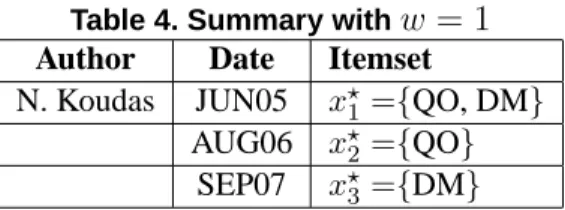
Let us give an illustration of a summary with our toy example. The representative sequences extracted from Table 3 are give Table 4. Here, we achieve the dual goal of numerosity reduction (from 6 events to
3) and domain reduction (from 6 descriptors to 2). These compression effects are obtained thanks to the user defined parameters, i.e., the generalization vectorϑand the temporal sliding windoww, that control the trade-off between resp. semantic accuracy vs. standardization and time accuracy vs. compression.
Table 4. Summary withw= 1 Author Date Itemset
N. Koudas JUN05 x⋆1={QO, DM}
AUG06 x⋆2={QO}
SEP07 x⋆3={DM}
4.6 The TSaR algorithm
From an operational view point, our implementation of TSaR is shown in Algorithm 1. The sum- mary is computed through an incremental algorithm that generalizes and appends incoming events one at a time into the current output summary. In other words, assume the current summary is s⋆M = χϑ,w(hx1, . . . , xni) = hπ(y1), . . . , π(yj)iand the incoming event is (xn+1, tn+1). The algorithm com- putesχϑ,w(hx1, . . . , xn, xn+1i)with a local update tos⋆M, i.e., changes are only made within the lastw groupsyj−w, . . . , yj.
More precisely, (xn+1, tn+1) is generalized into (x′n+1, tn+1) (line 6). Then, assuming we denote W ={yk},1≤j−w≤k ≤jthe set of groups that are included in temporal windoww, TSaR checks ifx′n+1 is included in a group yk ∈ W. x′n+1 is either incorporated into a groupykif its ϑ-generalized version satisfies the (Cont) condition (line 8 to 9), or it initializes a new group{(yj+1, t′j+1 =tn+1)}in W (line 11 to 14). Once all input events are processed, the lastwgroups contained inW are projected and added to the output summarys⋆M (line 18 to 20). The final output summary is then returned and/or stored in a database.
Memory footprint. TSaR requireswgroups to be maintained in-memory for summarizing the input time sequence. The algorithm’s memory footprint is finite (O(1)) and bound by the width of w and the average size m of an event’s set of descriptors. The overall process memory footprint is obtained by adding the cost necessary to maintain in-memory the output time sequence s⋆M and the taxonomies and/or hashtable index to compute descriptors’ generalization. However,s⋆M can be projected and written to disk at regular intervals. Therefore, TSaR’s overall memory footprint remains constant and limited compared to the amount of RAM now available on any machine.
Processing cost. TSaR performs generalization, grouping and concept formation on the fly for each incoming event. The process has an algorithmic complexity linear with the number of eventsO(n). The processing cost is weighted by a constant cost c = a∗b. ais the cost for generalizing an event’s set of descriptors and mainly depends on the number of taxonomies and their size. bis the cost to scan the finite list of groups inW. However,ais a cost that can be reduced by precomputing the generalization of each descriptive domain and storing the results in a hashtable index. bis a cost that is negligible since the temporal windowswused are small, e.g., mostlyw≤ 25in our experiments. Hence, we satisfy the memory and processing requirements presented earlier.
5 Experiments
In this section we validate our summarization approach through an extensive set of experiments on real-world data from Reuter’s financial news archives. First, we describe the data and how taxonomies are acquired for the descriptive domains of the news. We summarize the raw data with different temporal windows w and show the following properties of the TSaR algorithm: (i) low processing cost, (ii) linearity and (iii) compression ratio.
Algorithm 1 TSaR’s pseudo-code
1. INPUT:ϑ, taxonomiesH,w, time sequence of eventss
2. LOCAL:W FIFO list containing thewlast groups
3. OUTPUT: Summarys⋆M
4. for all incoming event(xn+1, tn+1)∈sdo
5. {// Generalization usingH}
6. x′n+1 ←ϕϑ(xn+1)
7. {// Grouping}
8. if∃(yk, t′k)∈W, wherex′n+1 ⊑ykthen
9. yk ←yk∪x′n+1{//x′n+1 is grouped intoyk}
10. else
11. if|W|> w{// Case whereW is full}then
12. PopW’s1st groupyj−w, addπ(yj−w)intos⋆M
13. end if
14. W ←W ∪ {(x′n+1, tn+1)} {// UpdatingW}
15. end if
16. end for
17. {// Add all groups inW intos⋆M}
18. whileW 6=∅do
19. PopW’s1st groupyi, addπ(yi)intos⋆M
20. end while
21. return s⋆M
Our experiments were performed on a Core2Duo 2.0GHz laptop, 2GB of memory, 4200rpm hard drive and running Windows Vista Pro. The DBMS used for storage is PostgreSQL 8.0 and all code was written in C#.
5.1 Financial news data and taxonomies
n financial applications, traders are eager to discover knowledge and eventual relationships between live news feeds and market data in order to create new business opportunities [30]. Reuters has been generating and archiving such data for more than 10 years. To experiment and validate our approach in a real-world environment, we used one year of Reuters’s news articles (2003) written in English. The unprocessed data set comes as a log of 21,957,500 entries where each entry includes free text and a set of≈ 30attribute-value pairs of numerical or categorical descriptors. An example of raw news event is given in Table 5. As provided by Reuters, the data can not be processed by the TSaR algorithm. Hence, the news data was cleaned and preprocessed into a sequence of events processable by TSaR.
Among all the information embedded in Reuters’s news articles we focused on 3 main components for representing the archive as a time sequence:
•Timestamp: This value serves for ordering a news article within a time sequence.
•Topic codes: When news articles are written, topic codes are added to describe their content. There are in total 715 different codes relating to 20 different topics. We used 7 of the most popular topics to describe the data, i.e., {Location, Commodities, Economy Central Banking and Institution, Energy, Equities, Industrial sector, General news}.
•Free text: This textual content is a rich source of information from which precise semantic descrip- tors can be extracted. Give 5 additional topics, namely,{Business, Operation, Economics, Government, Finance}, we used the WordNet [3] ontology to extract additional descriptors from this content.
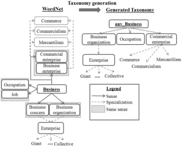
Figure 3. Taxonomy generated for thebusinessdomain
Table 5. Example of raw news event:
Timestamp 01 Jan 2004
Topic code EUROPE USA Bank INS NL
Free text Dutch bank ABN AMRO said on Wednesday it had reached a preliminary agreement to sell its U.S.-based Professional Brokerage business to Merrill Lynch & Co. . . . Extracting pertinent descriptors from free text is a non trivial task w.r.t. the need for organizing the de- scriptors extracted into taxonomies. Research in Natural Language Processing (NLP) could be leveraged to tag texts based on their corpus, e.g., using Term Frequency-Inverse Document Frequency (TF-IDF) weights as done in [12] or using online resources such as Open Calais [2]. However, creating taxonomies from the tags extracted is not trivial and requires prior knowledge on the descriptors. The paradox lies in the fact that these descriptors are not known in advance. We chose to use the WordNet [3] ontology as a guide for extracting descriptors and structuring them into taxonomies thanks to the hierarchical or- ganization already existing in WordNet. This choice leaves room for improvement by leveraging more complex techniques for both extracting descriptors from the free text and structuring these descriptors.
For example, automatic approaches [17] or hierarchical sources such as Wikipedia [22, 7] could also be used. However, such research is out of the scope of this paper.
In total, we preprocessed the input archive into a sequence of 1,283,277 news events.Each news event is described on the 12 descriptive domains selected earlier and several descriptors from each domain can be used. We generated a taxonomy for each of these descriptive domains. As the domains of topic code themes are limited in size and already categorized, corresponding taxonomies were manually generated.
Descriptive domains extracted from the free text were generated using the WordNet ontology as shown in Figure 3. In a nutshell, for a given subject, e.g., business, its senses are used as intermediary nodes in the taxonomy. If there are several synonyms for one sense, e.g., {Commercial enterprise, Business enterprise}, one is arbitrarily chosen, e.g., Commercial enterprise. Specialized descriptors are then used as lower level descriptors.
5.2 Summarization
The TSaR algorithm takes as input taxonomiesHA, a generalization vectorϑ, temporal window pa- rameter w and a time sequence. The expected output is a more concise representation of the input sequence where the descriptive domains and the number of input events are reduced.
5.2.1 Quality measure
The quality of the algorithm can be evaluated by different methods. First, we could evaluate the summarization algorithm w.r.t. the application that it is meant to support, e.g., Sequential Pattern Mining (SPM). In this case, the summary can be evaluated based on its ability to increase the quality of the output knowledge or increase the speed of the mining process (a preliminary study is proposed in our technical report [21]).
Second, we can measure the semantic accuracy of summarized event descriptors in the summary produced. This accuracy can be evaluated thanks to the ratioα = |Ω|Ω|′|, whereΩis the set of descriptors in the raw data and Ω′ is the set of generalized descriptors in the output summary. The higher α, the better the semantic accuracy.
In addition to the semantic accuracy of the summary, we can also measure its temporal accuracy. For this purpose, given a time sequence s = {xi}, 1 ≤ i ≤ n, temporal locality w > 1 and a temporal window W, we define a temporal rearrangement penalty cost for grouping an incoming event xi with a group yj ∈ W. We denote this penalty costCτ(xi). Cτ(xi)expresses the number of rearrangements necessary on the timeline so that event xi can be grouped with yi in window W. Cτ(xi) penalizes incoming eventsxi that are grouped with the older groups yi inW; on the other hand, ifyi is the most recent group inW, no penalty occurs. Cτ(xi)is formally defined as follows:
Cτ = 0, if(6 ∃yj ∈W, xi ⊑yj), or,(∃yj ∈W, xi ⊑yj and6 ∃k > j, yk ∈W) Cτ =m,1≤m≤w−1, if∃yj ∈W, xi ⊑yj andm=|{yk ∈W, k > j}|.
The total temporal rearrangement penalty cost for summarizing s into s⋆M, denoted Cτ(s⋆M), is then Cτ(s⋆M) = Pn
i=1Cτ(xi). This penalty cost should then be normalized so that our results are compara- ble. Hence, we choose to compute the relative temporal accuracy of the summaries. We normalize all temporal rearrangement cost by the maximum cost obtained in our experiments, i.e.,Cτ(χh3i,100(s)).
Finally, we also evaluate the summarization algorithm on its numerosity reduction capability by re- porting its compression ratio CR. CR is defined as: CR = 1− |s|s|−1⋆M|−1 where |seq|is the number of events in a time sequenceseq. The higherCR, the better. We decide to useCRas it was also used by Kiernan and Terzi’s in [16] and we weight theCRwith the summaries’ semantic and temporal accuracy, αandβ, respectively.
5.2.2 Experiment results
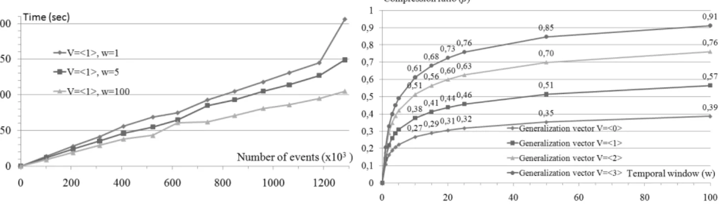
We start by setting the generalization vectorϑ = h1i, i.e., all descriptors are generalized once, and w∈ {1,2,3,4,5,10,15,20,25,50,100}where the maximum valuew= 100was chosen to represent a very strong temporal relaxation. Figure 4 gives the processing time of the TSaR algorithm with different temporal windows. For the sake of readability, we only display the plots for temporal windows w ∈ {1,5,100}. These plots show that the TSaR algorithm is linear in the number of input events for temporal windowswof any size. In addition, we can observe that processing times are almost constant whatever the temporal window considered. The slight variation observed in between different values ofwhave two complementary explanations. First, it is more costly to scan large windows during grouping. Second, a larger windowwallows to maintain more groups in-memory and, so, requires less I/O operations for writing into storage.
Table 6. Semantic accuracy
ϑ |Ω′| α h0i 1208 N/A h1i 50 1 h2i 20 0.40 h3i 13 0.26
We compute the CR of the summaries built with different generalization vectorsϑ ∈ {h0i,h1i,h2i,h3i}.
The results are given in Figure 5. Note that the best compression ratio achieved with ϑ = h0iis only 0.39. For a given temporal windoww, relaxing the precision of the data by generalizing each descriptor once, twice or three times allows an average gain in compression capabilities of 46.15%, 94.87% and 133.33% respectively. In other other words, the compression ratio is approximatively doubled when increasing the generalization level. Another interesting observation is that for allϑ, the plots show that highest numerosity reduction is achieved with larger temporal windows while processing times are al- most constant, as shown in Figure 4. This observation is very helpful from user view point for setting the summarization parametersϑandw. In effect, as processing times are almost constant whatever the temporal window considered, the user needs only to express the desired precision in terms of (i) seman- tic accuracy for each descriptive domain and (ii) temporal locality without worrying about processing times.
Table 6 gives the semantic accuracy of the summaries produced and Figure 6 gives their temporal accuracy. Note in Table 6 that the number of descriptors in the raw data, i.e.,ϑ = h0i, is 1208. When summarizing each descriptive domain once, i.e., ϑ = h1i, the number of descriptors in the summaries drops to 50. This loss of semantic information can be explained by the fact the data was preprocessed using the WordNet ontology and the taxonomies were also generated from the WordNet ontology. Nu- merous descriptors extracted from the free text are in fact synonyms and are easily generalized into one
common concept. Consequently, the concepts obtained withϑ=h1ishould be considered as better de- scriptors than the raw descriptors. Hence, we choose to computeαusing as baseline|Ω′|= 50, as shown in Table 6. In this case, each timeϑis increased, the semantic accuracy is approximatively halved. This observation is consistent with our previous observation on the average compression gain.
Figure 6 gives the relative temporal accuracy of each summary. Higher levels of generalization re- duce the temporal accuracy of the summaries. This phenomenon is due to the fact that more generic descriptors allow more rearrangements for grouping events. However, the temporal accuracy remains high, i.e.,≥0.80, for small and medium sized temporal windows, i.e.,w ≤25. The temporal accuracy only deteriorates with large windows, i.e.,w ≥ 25. This result means that the analyst can achieve high compression ratios without sacrificing the temporal accuracy of the summaries.
Figure 4. Processing time
Figure 5. Numerosity reduction
Figure 6. Temporal accuracy
However, guaranteeing theCR with TSaR is a difficult task, if not impossible, as its depend on the input parameters and on the data’s distribution. In addition, the analyst needs to weight the semantic and temporal accuracy he is ready to trade off for higherCR. Guaranteeing theCRbecomes an optimization problem that requires the algorithm to self-tune the input parameters and take into account the analyst’s preferences.
6 Conclusion and future work
Massive data sources appear as collections of time sequences of events in a number of domains such as medicine, the WWW, business or finance. A concise representation of these time sequences of events is desirable to support chronology-dependent applications. In this paper, we have introduced the concept of Time Sequence Summarization to transform time sequences of events into a more concise but informative form, using the data’s semantic and temporal characteristics.
We propose a Time Sequence SummaRization (TSaR) algorithm that transforms a time sequence of events into a more reduced and concise time sequence of events using a generalization, grouping and concept formation principle. TSaR expresses input event descriptors at higher levels of abstraction using taxonomies and reduces the size of time sequences by grouping similar events while preserving the overall chronology of events. The summary is computed in an incremental way and has an algorithmic complexity linear with the number of input events. The output is directly understandable by a human operator and can be used, without the need for desummarization, by chronology-dependent applications.
One such application could be conventional mining algorithms to discover high order knowledge. We have validated our algorithm by performing an extensive set of experiments on one year of Reuters’s financial news archives using our prototype implementation.
TSaR summaries are built using background knowledge in the form of taxonomies and the semantic and temporal precision of the output summary are controlled by user defined parameters. One direction in our future work is to render the generalization, grouping and concept formation process more flexible.
We would like to allow automatic tuning of the input parameters with regard to an objective to achieve, e.g., a compression ratio. The problem then turns into an interesting optimization issue between semantic accuracy vs. standardization and time accuracy vs. compression. Also, much research in the temporal databases and datastreaming have worked under the assumption that analysts are more interested in recent data and desire high precision representations for new data items while older data can become obsolete. Works in temporal databases have introduced the concept of decay functions to model ageing data. We would also like to extend TSaR in future work by introducing decay functions to further reduce descriptive domains and data compression of older or obsolete information.
7 Acknowledgements
We would like to thank Sherif Sakr, Juan Miguel Gomez and Themis Palpanas for their many helpful comments on earlier drafts of this paper. This work was supported by the ADAGE project, the Atlas- GRIM group, the University of Nantes, the CNRS and the region Pays de la Loire.
References
[1] Google finance. http://finance.google.com.
[2] Open calais. http://www.opencalais.com.
[3] Wordnet. http://wordnet.princeton.edu/.
[4] C. C. Aggarwal, J. Han, J. Wang, and P. S. Yu. On Clustering Massive Data Streams: A Summarization Paradigm, volume 31 of Advances in Database Systems, pages 9–38. 2007.
[5] S. Babu, M. Garofalakis, and R. Rastogi. Spartan: A model-based semantic compression system for massive data tables. In Proc. of SIGMOD, 2001.