La période de régularisation du modèle pourrait lisser toutes les inégalités et conduire à de mauvaises solutions sur les frontières des objets de la scène. L'idée ici est d'aborder le problème de la localisation des discontinuités dans la carte des disparités qui correspondent aux arêtes sur les objets du monde réel, ainsi que l'estimation des disparités.
Computational stereo vision
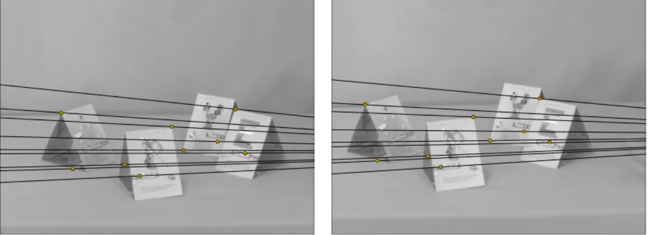
Epipolar constraint
All epipolar lines l in the left image pass through the epipole and similarly all epipolar lines l0 in the right image pass through e0. In terms of stereo correspondence, the epipolar geometry limits the search for the point corresponding to x to the linel0.
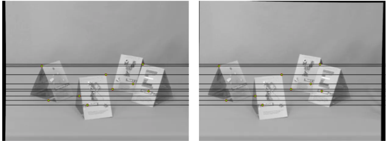
Rectification
That is, the search is reduced from sweeping the entire image to a 1D search along the epipolar line 10. This problem can be solved by transforming the left and right images so that the epipolar lines of the two are collinear and parallel to the horizontal axis.
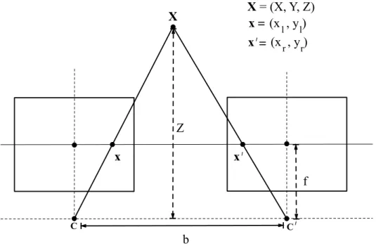
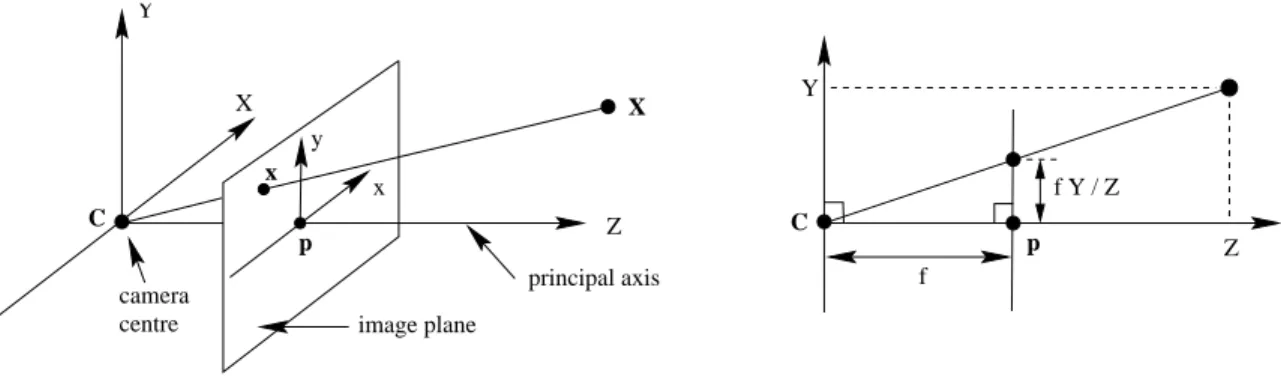
Disparity-depth relationship: Triangulation
Suppose that x = (xl, yl) is the point in the left image and x0 = (xr, yr) is the corresponding point in the right image. If we can now find the corresponding points in the two images, eg, x, x0, then we can find the disparity d and estimate the depth Z at the corresponding point in the 3D scene.
Methods for stereo correspondence
Using disparity maps and the intrinsic camera parameters, we can perform the 3D reconstruction of the scene. This prior distribution encodes the smoothness of the disparities, and the cost from the stereo image intensities is introduced as the probability.
Contributions of the thesis
Including only the stereo image intensities and smoothness term would model inequalities that may not be consistent with the geometric properties of the surface. This constraint leads to solutions consistent with the surface geometric properties of the scene.
Outline of the thesis
In Chapter 6, we summarize the methods proposed in the thesis and highlight some important aspects related to them. In the next section, we will briefly discuss some of the early stereo algorithms and their limitations.
Energy minimization-based algorithms
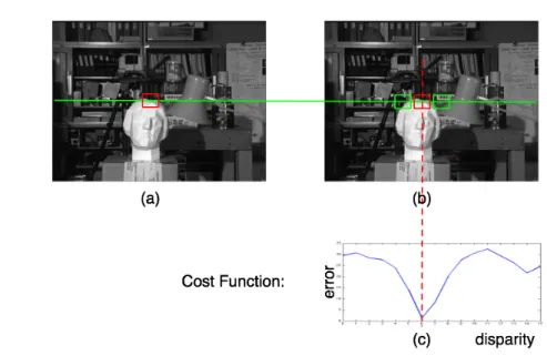
Energy function formulation
The definition of the interaction function Vx,y(dx, dy) is very important in determining the smoothness of the final disparity map. We will show how the minimization of an energy function is equivalent to finding the maximum posterior estimate of a given Markov random field (MRF).
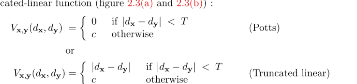
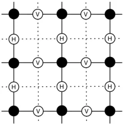
Markov Random Fields and stereo
- Disparity estimation as Labelling Problem
- MAP-MRF estimation
The probability function P(I|d) expresses how likely the observed data are for different disparity settings. Since Vx,y(dx, dy) determines the smoothness of the disparity map and is part of the prior (2.16), it also refers to the assmothness prior.
Optimization
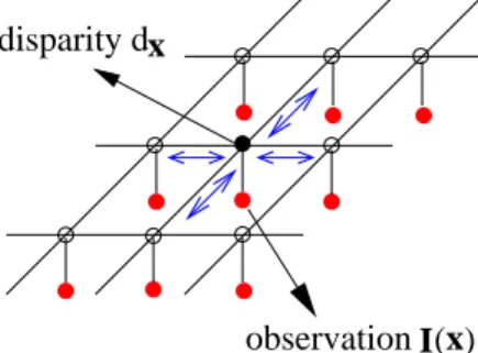
- Mean Field Approximation
- Belief Propagation
- Graph Cuts
- Other methods
A more detailed and in-depth comparison of the mean field and belief propagation is provided in the paper by Weiss [2001]. As stated by Szeliski et al., although there are a number of methods to optimize, the main requirement is actually to have an energy that is representative of the scene.
Additional cues and constraints
Occlusion handling: Additional binocular cues
The disparity map is represented by a path in the matched space, which is broken when a discontinuity is detected or when an occluded region occurs. Most recent algorithms model the occlusions taking into account the visibility of the point in the two images. That is, each correspondence is associated with a binary label that indicates whether a particular point is visible in the other image or not.
Localizing disparity discontinuities: Colour and gradient cues
Each of these hypotheses was then tested using a quality measure inferred from image distortion. Hong and Chen [2004] formulated the stereo matching problem as an energy minimization problem in the segment domain instead of the traditional pixel domain. Furthermore, they do not use over-segmentation through mean-shift filtering like most other segmentation-based approaches.
Disparity surfaces: Geometric constraints
They then relate these derivatives to differential properties of the surface, such as those encoded by normals and curvatures. Alternatively, Li and Zucker [2006a,b] explicitly take into account the differential geometric properties of the surface. These regularization weights are also the ones that determine the sparseness of the graph itself.
Motivation
Before going into the details of each of these models, we first provide a brief state-of-the-art on coupled random fields in the next chapter. The depth values for the surface must match the surface properties, such as surface normals, for the scene. Finally, in section 3.4, we present the highlights of the thesis with reference to coupled MRFs and Alternating Maximization.
Related work
Line process-based coupled-MRFs
The process of reconstruction consists of segmentation of the images using the line process and the confidence field. Again, the image intensities are modeled as a continuous field and the line process as a binary field. In the case of Sun et al., the three MRFs are used to represent disparity, discontinuity, line process, and occlusions.
Coupled-MRFs without line process
While the method of Nasrabadi et al. suggested only the enhancement of disparity information using optical flow, Sudhir et al. Referring to the example equation (3.1), if the optical flow is represented by the variable A, the band disparity and the observed images represented by I1 and I2. Each of these energies E1 and E2 include discontinuity information within the disparity and optical flow estimates respectively, based on the consistency between the right and left images given at two different time instances (I1 and I2).
Summary basic concepts of coupled-MRFs
Table 3.1: Summary of paired usage methods-paired MRFs-No. of General Energy Optimization Applications Variables Functions Optimization Techniques Surface Interpolation Line Process (LP) Metropolis Algorithm Marroquin [1984] and Surface Representation and Gradient Irosi Phase [1991], LPand Surface Deptoni SequentialMeanField GeigerandYuille[1991] Discontinuity Estimation LPand Image Characteristics Metropolis Algorithm GambleandPoggio[1987] like color, movement ,stereoone/ sequential modules for optical flow estimation HeitzandBouthemy[1993]LPandOpticalflowoneSequentialICM Acousticimageprocessing MurinoandTrucco[1998]LP,besimiandrangeoneSequentialSimulatedAnnealingSegmentationSegmentationWoneLP]nola equentialICM DisparityEstimationOcclusion-LP,Eliminate Sunetal.[2003]Discontinuity-LPone LineprocessesBP andDisparity Muti-targettrackingexistenceoftarget-LP, Elimino Xueetal .[ 2008]Occlusion-LPone LineprocessesBP and Multipletargets ImageRestorationMixedannealingSimulatedAnnealing Bedinietal.[2001]LPandimageintensityone LikeAlternation and Least Square Minimization Optical flux estimation of optical flux and disparity simulated annealing and segment labels.
Alternating Maximization
By using Bayes' theorem, it is very easy to show that the alternation in equation (3.7) corresponds to the following, So the above equation shows that the inference of each of the variables a and b can be done using only the conditional distributions p(a|b,I) and p(b|a,I) respectively. This greatly simplifies modeling, as there is no need to specify a completely common model.
Coupled-MRF in the proposed approach
The function of the displacement model is therefore to estimate the directions in which the discontinuities must be moved. The gradient map of the reference image (in our case the left image) is used as evidence for the object boundaries. The displacement values give the direction in which the disparity discontinuities must be moved to align with nearest maxima of the gradient magnitude.
Joint disparity and displacement model
Displacement conditional disparity model
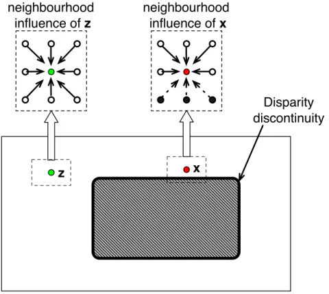
We first specify the disparity distribution conditional on the displacement field and the observed data, p(d|a,I). The data term is similar to that in classical disparity MRF models (Felzenszwalb and Huttenlocher [2006]), while the interaction term is modified to include the displacement information. For a given pixel location x, only some of the neighbors in Nx actually interact with x, depending on the displacement values.
Disparity conditional displacement model
The second term on the right-hand side of (4.17), is the product of the probabilities defined in the interruption chains. The first terms on the right-hand side of (4.18) are defined using a data term and an interaction term as specified below. Then, we determine the difference in the magnitude of the gradient between the current position and the selected points along the normal.

Optimization
Viterbi algorithm
As described in section 4.2.2, the Markov chain is constructed to find the second-order shear field values. To retrieve the sequence M∗ we need to keep track of the argument of the recursive equation above for each and We will now discuss this coarse-to-fine procedure in some detail before presenting the results of the proposed technique.
Multi-grid optimization
In this way, the probabilities at each level move closer to the fixed point more quickly and therefore converge more quickly. The idea is to find the inequality mapdl at each level for the sitesSl minimization of the energy, E(dl) = X. 4.40) This equation is the same as the energy within the exponential in (4.5), except that it is expressed in terms of the image grid displayed at coarseness level l. However, the displacement calculation at each resolution is performed independently of the other levels.
Alternating Maximization procedure
An important point is that the active neighborhood H(a) is constructed at each level for the correction of inequalities at discontinuities. The alternation is performed until a large percentage (in our experiments 90%) of the displacement values equals zero at each scale. This indicates that no more corrections for the inequalities are required and the inequality discontinuities now correspond to the object boundaries.
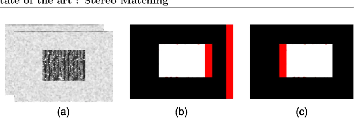
Experimental results
As can be seen in Figure 4.9(d), the discontinuities are unconformities at inappropriate locations but close to the actual object boundaries. The proposed cooperative approach using the gradient information (Figure 4.9(b)) can obtain the corrected disparity and object boundary map as shown in Figures 4.9(e) and 4.9(f), respectively. As can be seen in Figure 4.12(c), the standard mean-field algorithm, which only estimates the disparity information, does not give good results.
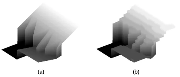
![Figure 4.8: Results on texture image: Shows evolution of the algorithm using the coarse-to- coarse-to-fine strategy suggested by Felzenszwalb and Huttenlocher [2006].](https://thumb-eu.123doks.com/thumbv2/1bibliocom/460719.67513/95.918.169.753.186.926/figure-results-evolution-algorithm-strategy-suggested-felzenszwalb-huttenlocher.webp)
Discussion
- Relationship between the normals in disparity and Euclidean space . 90
- Disparity model given the normals
- Discrete normal model given disparity
- Normal model without discretization
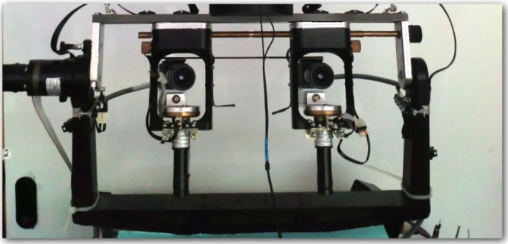
These chains in the objects arise due to the fronto-parallel assumption of the disparity MRF model. This is mainly done by taking into account the surface geometric properties of the objects in the scene. We specify the baseline, ie. the distance between the two camera centers, outside the focal length with f.

Overall optimization procedure
Experimental results
Comparing the performance of the two normal models
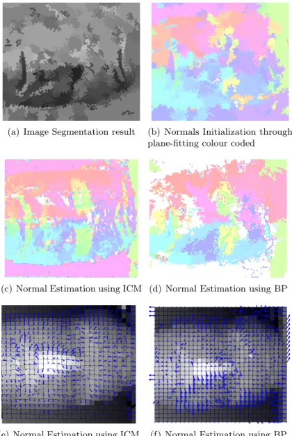
We see that the normals obtained using the ICM procedure are noisier compared to that of BP. The normals obtained using the surfnorm function in MATLAB are shown in Figure 5.7(b) as an arrow diagram. Figure 5.10 shows the results obtained using the normals obtained from the ICM and BP optimizations.
Further results using ICM-based normal estimation
Comparing the results of the normals using ICM and BP (Figures 5.11(c) and 5.11(d)), we see that the results obtained using the BP approach do not agree with the surface variations. Moreover, this estimation procedure also depends on the size of the regions obtained during the segmentation. Disparity and normals obtained for the main image using BP and ICM for normal estimation are shown in Figures 5.11(d) and 5.11(c).
Discussion
In the next section we provide a brief overview of the two models presented in this thesis. This allows us to find the position of the true boundary of the object based on the corrections applied to the discontinuities of the disparity. Inequality-CRF optimization was then performed using the standard mean-field algorithm.
Shared features of the two proposed approaches
The disparity-CRF was defined such that the interaction term includes derivatives of the first-order inequality, thereby forcing adjacent inequalities to lie in the same plane. However, this model requires dense discretization of normal space and therefore proved inefficient during optimization. The continuous model on the other hand provided a better alternative to the normal-CRF model.
Further directions of research
Stereo matching using iterative reliable disparity map expansion in color-spatial disparity space. This stereo matching task involves identifying the corresponding points in the left and right images, which are the projections of the same scene point. The aim of this thesis is to incorporate such constraints using monocular clues and differential geometrical information about the surface. To this end, this thesis considers two major problems associated with stereo tuning; the first is locating disparity discontinuities and the second is aimed at restoring binocular disparities according to the surface properties of the scene in question.
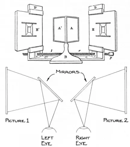
![Figure 1.2: Line drawings presented each eye through the stereoscope. Reproduced from Wheatstone [1838].](https://thumb-eu.123doks.com/thumbv2/1bibliocom/460719.67513/22.918.166.755.179.960/figure-line-drawings-presented-eye-stereoscope-reproduced-wheatstone.webp)
![Figure 1.6: Epipolar geometry images reproduced from the book by Hartley and Zisserman [2000].](https://thumb-eu.123doks.com/thumbv2/1bibliocom/460719.67513/27.918.153.763.186.477/figure-epipolar-geometry-images-reproduced-book-hartley-zisserman.webp)