HAL Id: tel-00666581
https://tel.archives-ouvertes.fr/tel-00666581
Submitted on 6 Feb 2012
HAL is a multi-disciplinary open access archive for the deposit and dissemination of sci- entific research documents, whether they are pub- lished or not. The documents may come from teaching and research institutions in France or abroad, or from public or private research centers.
L’archive ouverte pluridisciplinaire HAL, est destinée au dépôt et à la diffusion de documents scientifiques de niveau recherche, publiés ou non, émanant des établissements d’enseignement et de recherche français ou étrangers, des laboratoires publics ou privés.
Biology
Mauricio Labadie
To cite this version:
Mauricio Labadie. Reaction-diffusion equations and some applications to Biology. Adaptation and Self-Organizing Systems [nlin.AO]. Université Pierre et Marie Curie - Paris VI, 2011. English. �NNT :
�. �tel-00666581�
Th`ese de Doctorat
Sp´ecialit´e Math´ematiques
Ecole Doctorale de Math´ematiques de Paris Centre (ED386)
pr´esent´ee par Mauricio LABADIE
Reaction-Diffusion equations and some applications to Biology
Directeur:
Henri BERESTYCKI
Directeur d’´ etudes au CAMS-EHESS et CNRS
Soutenue le 8 d´ecembre 2011
avec des syst`emes et des ´equations de r´eaction-diffusion. La th`ese est divis´ee en sept chapitres:
• Dans le Chapitre 1 on mod´elise des ions de calcium et des prot´eines dans une ´epine den- dritique mobile (une microstructure dans les neurones). On propose deux mod`eles, un avec des prot´eines qui diffusent et un autre avec des prot´eines fix´ees au cytoplasme. On d´emontre que le premier probl`eme est bien pos´e, que le deuxi`eme probl`eme est presque bien pos´e et qu’il y a un lien continu entre les deux mod`eles.
• Dans le Chapitre 2 on applique les techniques du Chapitre 1 pour un mod`ele d’infection virale et r´eponse immunitaire dans des cellules cultiv´ees. On propose comme avant deux mod`eles, un avec des cellules qui diffusent et un autre avec des cellules fix´ees. On d´emontre que les deux probl`emes sont bien pos´es et qu’il y a un lien continu entre les deux mod`eles.
On ´etudie aussi le comportement asymptotique et la stabilit´e des solutions.
• Dans le Chapitre 3 on montre que la croissance a deux effets positives dans la formation de motifs ou patterns. Le premier est un effetanti explosion (anti-blow-up) car les solutions sur un domaine croissant explosent plus tard que celles sur un domain fix´e, et si la crois- sance est suffisamment rapide alors elle peut mˆeme empˆecher l’explosion. Le deuxi`eme est un effet stabilisant car les valeur propres sur un domaine croissant ont des parties r´eelles plus petites que celles sur un domaine fix´e.
• Dans le Chapitre 4 on ´etend la d´efinition de front progressif `a des vari´et´es et on en ´etudie quelques propri´et´es.
• Dans le Chapitre 5 on ´etudie des front progressifs sur la droite r´eelle. On d´emontre qu’il y a deux fronts progressifs qui se d´eplacent dans des directions oppos´ees et qu’ils se bloquent mutuellement, g´en´erant ainsi une solution stationnaire non-triviale. Cet exemple montre que pour des mod`eles `a diffusion non-homog`ene les fronts progressifs ne sont pas n´ecessairement des invasions.
• Dans le Chapitre 6 on ´etudie des fronts progressifs sur la sph`ere. On d´emontre que pour des sous-domaines de la sph`ere avec des conditions aux limites de Dirichlet le front progressif est toujours bloqu´e, tandis que pour la sph`ere compl`ete le front peut ou bien invahir ou bien ˆetre bloqu´e, tout en fonction des conditions initiales.
• Dans le Chapitre 7 on ´etudie un probl`eme elliptique aux valeurs propres nonlin´eaires.
Sur S1 on d´emontre l’existence de multiples solutions non-triviales avec des techniques de bifurcation. Sur SN on utilise les mˆemes arguments pour d´emontrer l’existence de multiples solutions non-triviales `a sym´etrie axiale, i.e. qui ne d´ependent que de l’angle vertical.
Mot Cl´es : Equations de r´eaction-diffusion, analyse nonlin´eaire, ´equations aux d´eriv´ees par- tielles paraboliques, ´equations aux d´eriv´ees partielles elliptiques, sur-solutions et sous-solutions, m´ethodes variationelles, m´ethodes topologiques, Biomath´ematiques.
The motivation of this PhD thesis is to model some biological problems using Reaction- diffusion systems and equations. The thesis is divided in seven chapters:
• In Chapter 1 we model calcium ions and some proteins inside a moving dendritic spine (a microstructure in the neurons). We propose two models, one with diffusing proteins and another with proteins fixed in the cytoplasm. We prove that the first problem is well-posed, that the second problem is almost well-posed and that there is a continuous link between both models.
• In Chapter 2 we applied the techniques of Chapter 1 for a model of viral infection of cells and immune response in cultivated cells. We propose as well two models, one with diffusing cells and another with fixed cells. We prove that both models are well-posed and that there is a continuous link between them. We also study the asymptotic behaviour and stability of solutions for large times, and we perform numerical simulations in Matlab.
• In Chapter 3 we show that growth has two positive effects on pattern formation. First, ananti-blow-up effect because it allows the solution on a growing domain to blow-up later than on a fixed domain, and if growth is fast enough then it can even prevent the blow-up.
Second, astabilising effect because the eigenvalues on a growing domain have smaller real part than those on a fixed domain.
• In Chapter 4 we extend the definition of travelling waves to manifolds and study some of their properties.
• In Chapter 5 we study travelling waves on the real line. We prove that there are two travelling waves moving in opposite directions and that they mutually block, giving rise to a non-trivial steady-state solution. This example shows that for models with non- homogeneous diffusion the travelling waves are not necessarily invasions.
• In Chapter 6 we study travelling waves on the sphere. We prove that for sub-domains of the sphere with Dirichlet boundary conditions the travelling wave is always blocked, but for the whole sphere the wave can either invade or be blocked, depending on the initial conditions.
• In Chapter 7 we study an elliptic nonlinear eigenvalue problem on the sphere. In S1 we prove the existence of multiple non-trivial solutions using bifurcation techniques. In SN we use the same arguments to prove the existence of multiple axis-symmetric solutions, i.e. depending only on the vertical angle.
Keywords : Reaction-diffusion equations, nonlinear analysis, parabolic partial differential equations, elliptic partial differential equations, super-solutions and sub-solutions, variational methods, topological methods, Biomathematics.
some applications to Biology
Mauricio Labadie 2011
Introduction vii
I Reaction-diffusion systems and modelling 1
1 Calcium ions in dendritic spines
Work in collaboration with Kamel Hamdache. Published in Nonlinear Analysis: Real World
Applications, Volume 10, Issue 4, August 2009. 3
1.1 Introduction . . . 3
1.1.1 Dendritic spines . . . 3
1.1.2 The role of Ca2+ in spine twitching and synaptic plasticity . . . 4
1.1.3 The original model . . . 5
1.2 The modified model and main results . . . 7
1.2.1 New variables . . . 7
1.2.2 Modeling the twitching motion of the spine . . . 8
1.2.3 The modified model . . . 9
1.2.4 Main results . . . 10
1.3 Proof of Theorem 1.1 . . . 12
1.3.1 A priori estimates . . . 12
1.3.2 The Fixed Point operator . . . 13
1.3.3 Conclusion of the proof . . . 17
1.4 Proof of Theorem 1.2 . . . 18
1.4.1 A priori estimates . . . 18
1.4.2 The Fixed Point operator . . . 19
1.4.3 Conclusion of the proof . . . 20
1.5 Proof of Theorems 1.3 and 1.4 . . . 22
1.5.1 Proof of Theorem 1.3 . . . 22
1.5.2 Proof of Theorem 1.4 . . . 23
1.6 Final remarks . . . 23
1.6.1 On the cytoplasmic flux . . . 23
1.6.2 On the diffusion coefficient . . . 24
1.6.3 On the reactions between calcium and the proteins . . . 24
1.7 Discussion . . . 24 iii
Work in collaboration with Anna Marciniak-Czochra. Already submitted. 27
2.1 Introduction . . . 27
2.1.1 Spatial effects of viral infection and immunity response . . . 27
2.1.2 The original model . . . 28
2.1.3 Biological hypotheses of the new model . . . 29
2.1.4 The reaction-diffusion (RD) model . . . 30
2.1.5 The hybrid model . . . 30
2.2 Main results . . . 30
2.2.1 Existence and uniqueness results . . . 31
2.2.2 Asymptotic results for the RD system . . . 31
2.2.3 Asymptotic results for the hybrid system . . . 32
2.3 Numerical simulations . . . 33
2.4 The fixed point operator and a priori estimates . . . 37
2.4.1 Construction of the fixed point operator R . . . 37
2.4.2 Positivity of solutions . . . 37
2.4.3 A priori estimates . . . 39
2.4.4 Continuity of the operator R . . . 41
2.5 Proof of the theorems . . . 43
2.5.1 Proof of Theorem 2.1 . . . 43
2.5.2 Proof of Theorem 2.2 . . . 44
2.5.3 Proof of Theorem 2.3 . . . 44
2.5.4 Proof of Theorem 2.4 . . . 45
2.5.5 Proof of Theorem 2.5 . . . 46
2.5.6 Proof of Theorem 2.6 . . . 53
2.6 Discussion . . . 55
II Reaction-diffusion equations and systems on manifolds 57 3 The effect of growth on pattern formation 59 3.1 Introduction . . . 59
3.2 Main results . . . 60
3.2.1 Reaction-diffusion systems on growing manifolds . . . 60
3.2.2 Properties of solutions: existence and uniqueness . . . 62
3.2.3 The anti-blow-up effect of growth . . . 63
3.2.4 The stabilising effect of growth . . . 66
3.3 Proof of Theorem 3.1 . . . 67
3.3.1 Parametrisation and Riemannian metric . . . 67
3.3.2 The general model with growth and curvature . . . 67
3.3.3 The isotropic growth model . . . 70
3.4 Proof of Theorem 3.2 . . . 70
3.5 Proof of Theorem 3.3 . . . 73
3.6 Proof of Theorem 3.4 . . . 73 iv
4.1 Definition of general travelling waves on manifolds . . . 79
4.1.1 Complete Riemannian manifolds . . . 79
4.1.2 Reaction-diffusion equations on manifolds . . . 80
4.1.3 Fronts, waves and invasions . . . 81
4.2 Properties of fronts on manifolds . . . 83
4.3 Proofs . . . 84
4.3.1 Proof of Theorem 4.1 . . . 84
4.3.2 Proof of Theorem 4.2 . . . 87
4.3.3 Proof of Theorem 4.3 . . . 89
5 Travelling waves on the real line 97 5.1 Introduction . . . 97
5.1.1 Calcium waves and fertilized eggs . . . 97
5.1.2 The reaction-diffusion model on the sphere . . . 98
5.1.3 Murray’s approach . . . 99
5.1.4 Modified equation . . . 100
5.1.5 On intuition and the real dynamics of the travelling waves . . . 100
5.2 Main results . . . 101
5.3 Proofs . . . 103
5.3.1 Supersolutions and subsolutions . . . 103
5.3.2 Global solution for N . . . 106
5.3.3 Global solution for S . . . 110
5.3.4 Steady-state solutions and blocking of the waves . . . 111
5.4 Discussion . . . 112
6 Travelling waves on the sphere Work in collaboration with Henri Berestycki and Fran¸cois Hamel. To be submitted. 113 6.1 Elliptic equation on the truncated sphere . . . 113
6.1.1 Trivial solutions . . . 115
6.1.2 Non-trivial solution: variational approach . . . 116
6.1.3 Pair of non-trivial solutions: topological approach . . . 118
6.2 Reaction-diffusion equations on the truncated sphere . . . 122
6.3 Elliptic equation on theN-sphere . . . 123
6.3.1 Trivial solutions . . . 123
6.3.2 Stability of solutions . . . 126
6.3.3 Non-trivial solutions . . . 127
6.4 Reaction-diffusion equation on theN-sphere . . . 129
6.4.1 Bistable nonlinearity . . . 129
6.4.2 Monostable nonlinearity . . . 132
6.5 Discussion . . . 136 v
III Elliptic equations and nonlinear eigenvalues on the sphere 139
7 Bifurcation and multiple periodic solutions on the sphere
Work in collaboration with Henri Berestycki and Fran¸cois Hamel. To be submitted. 141
7.1 Bifurcation onS1 . . . 141
7.1.1 Properties of solutions . . . 141
7.1.2 Proof of Conjecture 6.12 for S1 . . . 149
7.1.3 Bifurcation analysis . . . 149
7.2 Bifurcation onSN . . . 152
7.2.1 Eigenvalues and eigenvectors . . . 152
7.2.2 Groups, actions and equivariance . . . 153
7.2.3 Symmetries and reduction to an ODE . . . 154
7.2.4 Existence and uniqueness of axis-symmetric solutions . . . 155
7.2.5 Bifurcation analysis of axis-symmetric solutions . . . 156
7.3 Discussion . . . 158
IV Perspectives 161 8 Conclusions 163 8.1 Reaction-difusion systems and modelling . . . 163
8.1.1 Calcium dynamics in neurons . . . 163
8.1.2 Virus infection and immune response . . . 163
8.2 Reaction-diffusion equations and systems on manifolds . . . 164
8.2.1 The effect of growth on pattern formation . . . 164
8.2.2 Generalised travelling waves on manifolds . . . 165
8.2.3 Travelling waves on the real line . . . 165
8.2.4 Travelling waves on the sphere . . . 166
8.3 Elliptic equations and nonlinear eigenvalues on the sphere . . . 166
8.3.1 Bifurcation and multiple periodic solutions on the sphere . . . 166
References 169
The motivation of this PhD thesis is to model some biological problems using Partial Differential Equations. The general framework is a set of biological entities (either ions, molecules, proteins or cells) that interact with each other and diffuse within a given domain. Therefore, building our models via reaction-diffusion systems and equations seems quite natural.
This thesis is divided in seven chapters. The first two deal with reaction-diffusion systems on Euclidean spaces and modelling:
• Chapter 1. Calcium ions in dendritic spines (microstructures in the neuron).
• Chapter 2. Viral infection of cells and immune response.
The next four chapters deal with reaction-diffusion equations on manifolds:
• Chapter 3. The stabilising effect of growth on pattern formation.
• Chapter 4. Definition and properties of generalised travelling waves on manifolds.
• Chapter 5. Generalised travelling waves on the real line.
• Chapter 6. Generalised travelling waves on the sphere.
The last chapter deals with elliptic nonlinear eigenvalues on the sphere:
• Chapter 7. Bifurcation and multiple periodic solutions on the sphere.
In all seven cases we are interested in pattern formation and the role of geometry. We prove at least local existence of solutions, but in most cases we managed to find sufficient conditions for the solutions to be globally defined.
In Chapters 1 and 2 we prove that the models are well-posed problems (global existence, uniqueness and continuous dependence on initial data) and that the solutions are non-negative.
This implies that any numerical method used to approximate the solutions is robust. Moreover, in Chapter 2 we also characterised the asymptotic behaviour of the solutions, which permits to determine the stable states and the long term interaction of cells and viruses.
A recurrent finding is a link between pattern formation and geometry. In Chapter 3 we prove that growth has two effects on pattern formation. The first one is a stabilising effect:
vii
the eigenvalues of the operator on a growing domain are smaller than the eigenvalues on the corresponding fixed domain. The second one is an anti-blow-up effect: growth enhances the possibility of having time-global solutions. We prove that for scalar equations with quadratic nonlinearities, which exhibit blow-up on the fixed domain, the blow-up time on the growing domain occurs later. Moreover, if growth is fast enough the solutions are globally defined, i.e.
there is no blow-up at all.
In Chapters 5 and 6 we show that the geometry of the domain plays a crucial role in the propagation of a travelling wave. Indeed, unlike classical planar travelling waves that invade the whole Euclidean space, on the sphere the travelling waves do not necessarily invade the whole domain. More precisely, we prove existence of generalised travelling waves that are eventually blocked by non-trivial steady-state solutions, which implies that the wave cannot invade the whole sphere. Since we find the same result on the projection of the sphere to the plane, on a truncated sphere and on the whole sphere, the geometry of the sphere plays an important role in the invasive nature of the travelling front.
In Chapter 7 we deal with an elliptic nonlinear eigenvalue problem on the sphere. In the case of S1 we prove via topological bifurcation the existence of multiple non-trivial solutions.
In the case ofSN we use the same arguments to prove the existence of multiple axis-symmetric solutions, i.e. solutions depending only on the vertical angle, thus independent on the horizontal angles.
Chapter 1. Calcium ions in dendritic spines
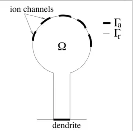
The study of synapses is a very recurrent and important topic that lies in the intersection of Medicine, Neurology, Biology and Chemistry. The current technology of microscopes has shown that the dendritic spines, the smallest structures of the neuron and the part responsible of the synapses, possess a twitching motion. The goal of our model is to propose a theoretical frame- work for this twitching motion and incorporate it into the dynamics of the calcium ions inside the neuron.
The motivation of Chapter 1 is the two articles of Holcman and his collaborators, [33] and [34]. In the former they use a stochastic model for each single calcium ion, whilst in the lat- ter they pass from the microscopic description to a macroscopic reaction-diffusion model via Fokker-Planck equations and the Law of Mass Action. This reaction-diffusion models describe the twitching motion of the dendritic spine, but the assumptions on the mechanism that triggers such twitches are not very realistic. After reviewing the experimental evidence in the literature (e.g. Farah et al [19], Klee et al [36] and Shiftman et al [59]), we propose to modify the hy- potheses on the genesis of the twitching to obtain a more accurate model from the biological point of view. With the new boundary conditions the problem is very nonlinear and strongly coupled, but we still have a well-posed problem.
We consider calcium ions interacting with some proteins that have 4 binding sites for the
full of cytoplasm. Let M be the concentration of calcium ions, U the total number of binding sites andW the total number of free sites andV the cytoplasmic flow field. If we suppose that the proteins are fixed in the cytoplasm (i.e. they do not diffuse) then the model is
∂tM = ∇ ·[D∇M−VM]−k1M U+k−1[A−U],
∂tU = −k1M U+k−1[A−U], V = ∇φ , △φ= 0.
(0.1) with initial conditions
M(x,0) = m0(x),
U(x,0) = A(x), (0.2)
and boundary conditions
M(σ, t) = 0 on Γa×[0, T], (D∇M−VM)·n(σ, t) = 0 on Γr×[0, T],
∇φ·n(σ, t) = a(σ)λ(t) on Γ×[0, T],
(0.3) where Γ :=∂Ω, Γ = Γa∪Γr and Γa∩Γr =∅. If we allow the diffusion of proteins then (0.1)-(0.3)
becomes
∂tM = ∇ ·[D∇M −VM]−k1M U+k−1W ,
∂tU = d△U−k1M U +k−1W ,
∂tW = d△U+k1M U −k−1W , V = ∇φ , △φ= 0.
(0.4)
with initial conditions
M(x,0) = m0(x), U(x,0) = A(x), W(x,0) = 0,
(0.5) and boundary conditions
M(σ, t) = 0 on Γa×[0, T], (D∇M−VM)·n(σ, t) = 0 on Γr×[0, T],
∇U·n(σ, t) = 0 on Γ×[0, T],
∇W ·n(σ, t) = 0 on Γ×[0, T],
∇φ·n(σ, t) = a(σ)λ(t) on Γ×[0, T].
(0.6)
Note thatdshould be much smaller than Dbecause the proteins we are considering are around 106 times bigger than the calcium ions.
The main results of the calcium ion problem is that both models admit weak, positive solutions and that there is a continuous link between both models. More precisely, we have the following three results.
Theorem 0.1 For any T >0 the reaction-diffusion system (0.1)-(0.3) has global unique weak solutionsM(x, t), U(x, t) and V(x, t) onΩ×(0, T) with the following properties:
1. M ∈L∞(Ω×(0, T)) and 0≤M(x, t)≤ km0k∞+k−1tkAk∞ a.e. inΩ×(0, T).
2. M ∈L∞ 0, T;H1(Ω) and kM(t)k2+D
Z t
0
eC(t−s)k∇M(s)k2ds≤eCt
km0k2+k−12 tkAk2 .
3. U ∈L∞(Ω×(0, T))and 0≤U(x, t)≤A(x) a.e. in Ω×(0, T).
4. V ∈L∞ 0, T;
L2(Ω)n
and kVkL∞(0,T;[L2(Ω)]n)≤Ckak∞kAk∞.
Theorem 0.2 For any T > 0 the reaction-diffusion system (0.4)-(0.6) is well-posed, i.e. it has global unique weak solutionsM(x, t),U(x, t), W(x, t) and V(x, t) on Ω×(0, T) depending continuously on the initial data. Moreover, we have the following properties:
1. M ∈L∞(Ω×(0, T)) and 0≤M(x, t)≤ km0k∞+k−1tkAk∞ a.e. inΩ×(0, T).
2. M ∈L∞ 0, T;H1(Ω) and kM(t)k2+D
Z t
0
eC(t−s)k∇M(s)k2ds≤eCt
km0k2+k−12 tkAk2 .
3. U, W ∈L∞(Ω×(0, T)), they are non-negative and 0≤U(x, t) +W(x, t)≤A(x) a.e. in Ω×(0, T).
4. U, W ∈L∞ 0, T;H1(Ω) and kU(t)k2+kW(t)k2+ 2d
Z t
0
eRstc(r)dr k∇U(s)k2+k∇W(s)k2
ds≤eR0tc(s)dskAk2, where c(t) = 2[k−1+k1α(t)] and α(t) =km0k∞+k−1tkAk∞.
5. V ∈L∞ 0, T;
L2(Ω)n
and kVkL∞(0,T;[L2(Ω)]n)≤Ckak∞kAk∞
Theorem 0.3 Ifd→0then the sequence(Md, Ud, Wd,Vd)of solutions of (0.4)-(0.6) converges to the solution(M, U, W,V) of (0.1)-(0.3) in the following senses:
1. Md,Ud andWd converge weakly in L2 0, T;L2(Ω)
to M, U and W, respectively.
2. Vd converges to V weakly in L2 0, T;
L2(Ω)n . 3. Md converges strongly in L2 0, T;L2(Ω)
toM.
4. Ud and Wd converge weakly-⋆ in L∞(Ω×(0, T))to U andW, respectively.
Finally, the solutions of both systems (0.1)-(0.3) and (0.4)-(0.6) are globally defined in time.
Theorem 0.4 Let M, U,W and V be solutions of either (0.1)-(0.3) or (0.4)-(0.6). Then:
1. M, U, W ∈L∞ 0,∞;L1(Ω) . 2. V ∈L∞ 0,∞;
L2(Ω)n .
Chapter 2. Viral infection and immune response
Starting from the assumption that cells and viruses diffuse and interact with each other moti- vates the framework of a reaction-diffusion system for viruses, normal cells and infected cells. If we add an immune response via antibodies then we should add as well a new type of cells that become resistant to viruses when they get in contact with antibodies. Models of this kind are important because of their potential applications in Cellular Biology and molecular transport, and could shed a light towards new gene therapies.
Getto et al [24] constructed an Ordinary Differential Equation model for virus infection of cells and immune response. The authors completely solved the model, and in particular they found that in the limit the viruses and the non-infected cells cannot coexist. Motivated by this result, we built up a reaction-diffusion model in order to study the spatial structure and properties of the solutions. Since the boundary conditions we imposed are homogeneous Neumann (i.e. no-flux), the problem is significantly easier than the one in Chapter 1 (calcium ions), which allows a complete description of the asymptotic behaviour and stability of solutions.
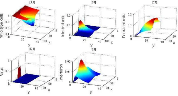
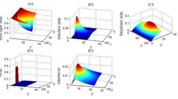
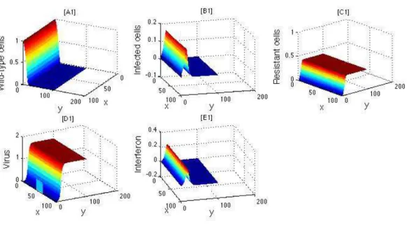
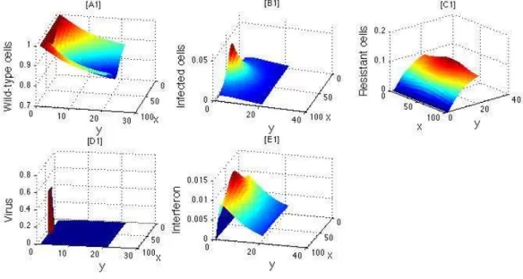
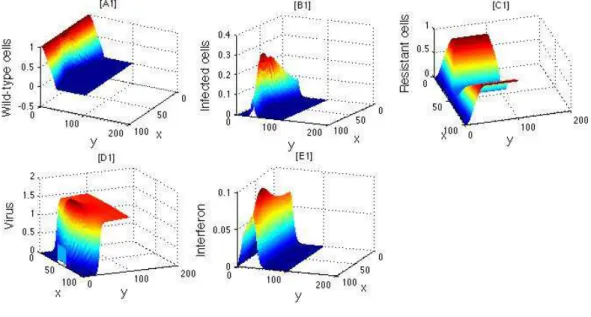
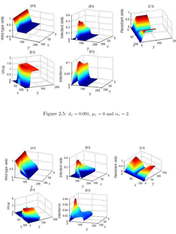
We consider a model where virions (i.e. viral particles)v infect cells, but we add an immune response from the organism via interferons i. There are 3 possible types of cells: wild-type cells W that has not been in contact with virions, infected cells I that have been in contact with virions, and resistant cellsR that have been in contact with interferons. All five biological particles are confined within a domain Ω with no-flux boundary conditions.
As in the calcium ion problem, we will consider two models. The first model is a reaction- diffusion (RD) system, where we allow cells to diffuse:
∂tW = d∆W −iW −vW ,
∂tI = d∆I−µII+vW ,
∂tR = d∆R+iW ,
∂tv = dv∆v−µvv+αvI −α4vW ,
∂ti = di∆i−µii+αiI−α3iW ,
(0.7)
with boundary conditions
∇W ·n(σ, t) = 0 on Γ×[0, T],
∇I·n(σ, t) = 0 on Γ×[0, T],
∇R·n(σ, t) = 0 on Γ×[0, T],
∇v·n(σ, t) = 0 on Γ×[0, T],
∇i·n(σ, t) = 0 on Γ×[0, T],
(0.8)
and initial conditions
W(x,0) = W0(x), I(x,0) = I0(x), R(x,0) = R0(x),
v(x,0) = v0(x). i(x,0) = i0(x).
(0.9)
In the second model we consider that the cells do not diffuse at all. Therefore, we set d= 0 and we thus obtain a hybrid model consisting of PDE equations for the interferonsiand virions v and ODE equations for the three types of cellsW, I, R:
∂tW = −iW −vW ,
∂tI = −µII+vW ,
∂tR = iW ,
∂tv = dv∆v−µvv+αvI −α4vW ,
∂ti = di∆i−µii+αiI−α3iW ,
(0.10)
with boundary conditions
∇v·n(σ, t) = 0 on Γ×[0, T],
∇i·n(σ, t) = 0 on Γ×[0, T]. (0.11) We prove that both the RD and the hybrid models are well-posed problems, i.e., they have unique solutions which are non-negative, uniformly bounded, and depend continuously on the initial data. We also prove that there is a “continuous link” between these two models.
Theorem 0.5 Fix any T >0. If the initial conditions (0.9) are non-negative a.e. and bounded then the RD system (0.7)-(0.8) has unique weak solutions W(x, t), I(x, t), R(x, t), v(x, t) and i(x, t)onΩ×[0, T]. Moreover, these solutions are non-negative, uniformly bounded, and depend continuously on the initial data.
Theorem 0.6 Fix any T >0. If the initial conditions (0.9) are non-negative a.e. and bounded then the hybrid system (0.10)-(0.11) has unique weak solutions W(x, t), I(x, t), R(x, t), v(x, t) and i(x, t) on Ω×[0, T]. Moreover, these solutions are non-negative, bounded, and depend continuously on the initial data.
converge to the solution(W, I, R, v, i)of the hybrid system (0.10)-(0.11), in the following sense:
• Strongly in L2 0, T;L2(Ω) .
• Weakly in L2 0, T;H1(Ω) .
• Weakly-⋆ in L∞(Ω×(0, T)).
So far we have (essentially) the same results we got for the calcium ion problem. However, the viral infection problem is easier because the boundary conditions are Neumann homogeneous, whilst for the calcium ions the boundary conditions were strongly coupled. This feature has allowed us to study in detail the asymptotic behaviour of solutions.
Theorem 0.8
1. The solutions W, I, R, v, i of the RD system (0.7)-(0.8) are globally-defined and belong to L∞(Ω×(0,∞)).
2. If W, I, R, v, i are non-negative, steady-state solutions of the RD system (0.7)-(0.8) then W(x) = W0≥0 constant,
I(x) ≡ 0,
R(x) = R0≥0 constant, v(x) ≡ 0,
i(x) ≡ 0.
Theorem 0.9 IfW, I, R, v, iare non-negative, steady-state solutions of the hybrid system (0.10)- (0.11) then
I(x) ≡ 0, v(x) ≡ 0, i(x) ≡ 0.
Moreover, suppose that the initial conditions belong to L∞(Ω). Then the solutions of the hybrid system (0.10)-(0.11) are globally-defined and have the following asymptotic properties:
1. I(x, t) belongs toL1(0,∞;L2(Ω)), i.e.,
t→∞lim Z t
0
Z
Ω
I2(x, s)dΩds <∞.
2. v(x, t) and i(x, t) belong to L1(0,∞;H1(Ω)), i.e.,
t→∞lim Z t
0
Z
Ω
v2(x, s)dΩ + Z
Ω|∇v(x, s)|2dΩ
ds <∞,
t→∞lim Z t
0
Z
Ω
i2(x, s)dΩ + Z
Ω|∇i(x, s)|2dΩ
ds <∞.
3. v(x, t)W(x, t) and i(x, t)W(x, t) belong to L1(0,∞;L1(Ω)), i.e.,
t→∞lim Z t
0
Z
Ω
v(x, s)W(x, s)dΩds <∞ and lim
t→∞
Z t
0
Z
Ω
i(x, s)W(x, s)dΩds <∞. 4. For any x∈Ω,
t→∞lim I(x, t) = 0, lim
t→∞v(x, t) = 0, lim
t→∞i(x, t) = 0. 5. For any x∈Ω, W0(x)>0 if and only if
t→∞lim W(x, t)>0.
Theorem 0.10 Consider the hybrid system (0.10)-(0.11) and suppose that µv = 0. Then:
1. If v∞(x) is a steady-state solution thenk∇v∞k= 0.
2. Define
v∞(x) := lim sup
t→∞ v(x, t).
If αv ≥α4µI then Z
Ω
v∞(x)dΩ≥ Z
Ω
v0(x)dΩ.
In particular, if v06≡0 thenv∞6≡0.
Chapter 3. The effect of growth on pattern formation
The study of pattern formation lies in the possibility of predicting the generation of certain patterns as a consequence of other factors, e.g. the strength of external stimuli and the concen- tration and diffusion of certain molecules. In Chapter 3 we focus our attention on the effect of growth in the existence and stability of patterns.
The study of pattern formation in reaction-diffusion systems started with the seminal paper of Turing [66], where he showed that the diffusion, a process that has a regularising effect, can drive instabilities when there are several substances interacting.
cent. In 1995 Kondo and Asai [38] reproduced numerically the skin patterns of a tropical fish by adding growth to the classical reaction-diffusion system. In 1999 Crampinet al [15] showed in 1D that the domain growth may increase the robustness of patterns. In 2004 Plazaet al [52]
derived a reaction-diffusion model for two morphogens on 1D and 2D growing, curved domains.
In 2007 Gjiorgjieva and Jacobsen [28] found that on a 2D sphere the solutions under slow growth are very similar to the solutions of the 2001 model of Chaplainet al [13] on a fixed sphere. They also showed numerically that the eigenmodes on the growing domain are smaller than those on the corresponding fixed domain, and that there is a continuous link between both patterns.
In Chapter 3 we prove that growth has two effects: (i) a regularising, anti-blow-up effect in the sense that growth not only delays the blow-up but it can even prevent it, and (ii) a stabilising effect in the sense that the eigenvalues of the linearisation on a growing domain have smaller real parts than those on a fixed domain.
Let Mbe ann-dimensional manifold without boundary and consider the reaction-diffusion system
∂u
∂t =D∆Mu+F(u), D=
D1
D2 . ..
DM
, Dk>0, (0.12)
where ∆M is the Laplace-Beltrami operator. Since we are interested in the effect of growth on pattern formation, we will consider (0.12) on a growing domain (Mt)t≥0. In particular, for isotropic growth we will assume that there is a growth functionρ(t) such thatMt:=ρ(t)M.
Our first result characterises generic reaction-diffusion systems on a growing manifold.
Theorem 0.11 Let(Mt)t≥0 be a growing manifold with metric(gij(ξ, t)). Under the hypotheses of Fick’s law of diffusion and conservation of mass, any reaction-diffusion system on Mt has the form
∂tu=D∆Mtu−∂t[logp
g(ξ, t) ]u+F(u), g:=det(gij), (0.13) where ∆Mt is he Laplace-Beltrami operator on Mt. In the case of isotropic growth we have
∂tu= D
ρ2(t)∆Mu−nρ(t)˙
ρ(t)u+F(u), (0.14)
where the coefficients of ∆M do not depend on time.
We prove local existence, uniqueness and regularity of solutions of (0.14). Moreover, under extra assumptions on the nonlinearity we prove that the solutions are global.
Theorem 0.12 There is a timeT >0such that the reaction-diffusion system (0.14) with initial conditionu0∈C
M,RM
has a unique solution u(t)∈C [0, T], C
M,RM .
Theorem 0.13 If F:RM →RM is C∞ then u(t)∈C∞
M ×(0, T],RM .
Theorem 0.14 Let (Mt)t≥0 be an isotropic growing manifold with growth rate c(t) :=nρ(t)˙
ρ(t) >0.
Suppose that the initial condition u0 of the reaction-diffusion system (3.4) is in C
M,RM and takes its values inside the rectangle R = (−1,1)M. Suppose further that for all (z, t) ∈
∂R ×[0,∞) we have
F(z)·n(z)< c(t), (0.15)
where n(z) is the outer normal at z. Then the solution u(t) of (0.14) is global and bounded, i.e. it exists for all timest≥0 and takes its values inside R. In particular, here is no blow-up whenever (0.15)holds.
From Theorem 0.14, if the growth rate is sufficiently big to satisfy c(t)>sup{kF(z)k:z∈∂R}
then the solution is globally bounded, which implies that there is no blow-up. Notice that since the growth ratec(t) is increasing inn, which implies that the dimension of the space enhances the regularity of solutions.
We quantitatively asses this anti-blow-up effect of growth for scalar equations. For homo- geneous equations we compare the corresponding ODE with and without growth. On the one hand, the ODE on a fixed domain is
u˙ =u2,
u(0) =u0>0, whose solution is
u(t) = 1
u0 −t −1
,
which blows up whent→t1 := 1/u0. On the other hand, the ODE on a growing domain is u˙ =−c(t)u+u2,
u(0) =u0>0, whose solution is
u(t) = Z t
0
ds ρn(s) ×
1 u0 −
Z t
0
ds ρn(s)
−1
,
Z t2
0
dt ρn(t) = 1
u0
.
It is easy to show that (i) t2 > t1 := 1/u0, (ii) t1 and t2 are decreasing functions of the initial condition u0, (iii) t2 is an increasing function on the spatial dimension n, and (iv) if growth is sufficiently fast, i.e. if the growth functionρ(t) satisfies
Z ∞ 0
dt ρn(t) ≤ 1
u0 thent2 =∞, i.e. there is no blow-up on the growing domain.
The same results hold for non-homogeneous scalar equations. Indeed, consider the scalar reaction-diffusion equation
∂tu = 1
ρ2(t)∆Mu−c(t)u+u2, u(0, ξ) = u0(ξ)>0.
If we define
η(t) :=
ZZ
M
u(t, ξ)dΩ, η(0) = ZZ
M
u0(ξ)dΩ>0. it can be shown that
η(t)≥ Z t
0
ds ρn(s)×
1 η(0) −α
Z t
0
ds ρn(s)
−1
. In particular, for an exponential growthρ(t) =ert such that nr > αη(0), i.e.
r > |M|
n ZZ
M
u0(ξ)dΩ,
we have blow-up on the fixed manifold but not on the growing manifold.
Besides the anti-blow-up effect of growth, there is a second effect that we found: under isotropic regimes, we proved that growth has a stabilizing effect on pattern formation, as the next theorem shows.
Theorem 0.15 Let (Mt)0≤t≤T be an isotropic growing manifold with growth rate c(t). Define S:=MT and notice that we will use the notation S for the fixed manifold andMT for the final stage of the growing manifold (Mt)0≤t≤T. Then λ is an eigenvalue of the reaction-diffusion operator on S,
LS := D
ρ2(T)∆S+dF(0)
if and only if λ−c(T) is an eigenvalue of the corresponding operator onMT, LMT := D
ρ2(T)∆MT −c(T)I+dF(0).
Theorem 3.5 says that when we compare the spectra of LS and LMT on the same manifold S=MT we obtain
spectrum(LMT) = spectrum(LS)−c(T).
Therefore, growth shifts the eigenvalues to the left in the complex plane, which is indeed a stabilising effect since the real parts are smaller. Moreover, this shift is exactly the growth rate c(T) > 0, which implies that the faster growth is, the more stable the patterns are. It is important to remark that, as far as we know, Theorem 3.5 is the first analytic proof of the stabilising effect of growth on pattern formation. It is worth to mention that the proof we provide does not hold for the case of non-isotropic growth.
Chapter 4. Generalised travelling waves on manifolds
We extend the current definitions of travelling waves in Euclidean spaces to curved domains, i.e.
to manifolds. This extension permits a unified framework to study the emergence and stability of patterns on manifolds, which is the main objective of Chapters 5, 6 and 7.
The study of travelling waves started in 1937 with the pioneering article of Kolmogorov [37]. Later on, in 1977 Aronson and Weinberger [3] proved the existence of multi-dimensional travelling waves, and in 1978 Fife and McLeod [20] proved that the travelling waves have an exponential decay at infinity. However, for the planar travelling waves to exist it is necessary to have an axis in the domain such that the equation is invariant under translations on that axis.
For non-planar travelling waves there are several approaches, but they could be divided in two categories: equations with coefficients that are not invariant under translations (i.e. in- homogeneous media) or domains that do not have an invariant direction (e.g. Euclidean domains with holes). For the study of such generalised travelling waves we refer the reader to Berestycki and Hamel [6], [7], [8] and Berestyckiet al [9], .
Berestycki and Hamel [8] defined a generalised travelling wave in terms of their level sets, which are no longer hyper-plans but hyper-surfaces. We realised that the definitions and prop- erties of generalised travelling waves were easily extended to the case of curved domains, i.e.
manifolds. We adapted the existing proofs for on general Euclidean domains and found that all the conclusions of Berestycki and Hamel [8] hold for complete, unbounded, Riemannian mani- folds.
It is worth to mention that of these results are straightforward, e.g. maximum principles and Harnack’s inequality, because they are local in nature. However, for global results such as a priori estimates we need uniform bounds of the coefficients.
LetMbe a complete, unbounded, Riemannian manifold and consider the reaction-diffusion
equation
∂tu=D∆Mu+F(t, x, u) ; t∈R, x∈ M,
u(0, x) =u0(x) ; x∈ M. (0.16)
are:
• EitherF is C1 and both F and ∂uF are globally bounded, or
• EitherF is bounded, continuous in (t, x) and locally Lipschitz continuous in u, uniformly in (t, x).
The goal of this project is to extend the notion of a travelling wave to manifolds. We start with several definitions. For any two subsetsA, B⊂ M denote
d(A, B) := inf{d(x, y) : x∈A, y ∈B}, whered(·,·) is the geodesic distance.
Definition 0.1 Ageneralised profileis a family (Ω±t ,Γt)t∈Rof subsets of Mwith the follow- ing properties:
1. Ω−t and Ω+t are non-empty disjoint subsets ofM, for anyt∈R. 2. Γt=∂Ω−t ∩∂Ω+t and M= Γt∪Ω−t ∪Ω+t, for any t∈R.
3. sup{d(x,Γt) : t∈R, x∈Ω−t}= sup{d(x,Γt) : t∈R, x∈Ω+t }= +∞
Suppose that there exist p−, p+ ∈ Rsuch that F(t, x, p±) = 0 for all t∈R and allx ∈ M. Thenu≡p± are solutions of (0.16).
Definition 0.2 Let u(t, x) be a time-global classical solution of (4.1) such that u 6≡p±. Then u(x, t) is ageneralized frontbetween p− and p+ if there exists a generalized front (Ω±t,Γt)t∈R
such that
|u(t, x)−p±| →0 uniformly whenx∈Ω±t and d(x,Γt)→+∞.
Definition 0.3 Let u(t, x) be a generalized front. We say that p+ invades p− or that u(t, x) is a generalised invasion of p− by p+ (resp. p− invades p+ or that u(t, x) is a generalised invasion ofp+ by p−) if
(i) Ω+t ⊂Ω+s (resp. Ω−s ⊂Ω−t ) for all t≤s.
(ii) d(Γt,Γs)→+∞ when |t−s| →+∞.
Definition 0.4 A generalised front u(t, x) has global mean speed c > 0 if the generalised profile(Ω±t ,Γt,)t∈R is such that
d(Γt,Γs)
|t−s| →c when|t−s| →+∞.
For anyx∈ M and any r >0 define
B(x, r) = {y∈ M : d(x, y)≤r}, S(x, r) = {y∈ M : d(x, y) =r}. We exhibit some properties of the level sets.
Theorem 0.16 Let p− < p+ and suppose that u(t, x) is a time-global solution of (0.16) such that
p−< u(t, x)< p+ for all (t, x)∈R× M.
1. Suppose u(t, x) is a generalised front between p− and p+ (or between p+ and p−) with the following properties:
(a) There exists τ >0 such that sup{d(x,Γt−τ) : t∈R, x∈Γt}<+∞, and
(b) sup{d(y,Γt) : y ∈ Ω±t ∩S(x, r)} → +∞ when r → +∞, uniformly in t ∈ R and x∈Γt.
Then:
(i) sup{d(x,Γt) : u(t, x) =λ}<+∞ for all λ∈(p−, p+).
(ii) p−<inf{u(t, x) : d(x,Γt)≤C} ≤sup{u(t, x) : d(x,Γt)≤C}< p+ for all C≥0.
2. Conversely, if (i) and (ii) hold for a certain generalised profile (Ω±t ,Γt,)t∈R and there existsd0 >0 such that for all d≥d0 the sets
{(t, x)∈R× M : x∈Ω±t, d(x,Γt)≥d}
are connected, then u(t, x) is a generalised front between p− and p+ (or between p+ and p−).
We prove that the global mean speed is unique and that generalised fronts are monotonic in time.
Theorem 0.17 Let p− < p+ and suppose that u(t, x) is a generalised front between p− andp+, where its associated profile (Ω±t ,Γt,)t∈R satisfies (b) in Theorem 0.16. If u(t, x) has a global mean speed c > 0 then it is independent of the generalised profile. In other words, if for any other generalised profile ( ˜Ω±t ,Γ˜t,)t∈R satisfying(b) the generalised front u(t, x) has global mean speed ˜c, then ˜c=c.
Theorem 0.18 Monotonicity
Let p−< p+ and supposeF(t, x, u) satisfies the following conditions:
(β) There existsδ >0such thatq7→F(t, x, q)is non-increasing for allq∈R\(p−+δ, p+−δ).
Let u(t, x) be a generalised invasion of p− by p+ and assume (as in Theorem 0.16) that:
(a) There exists τ >0 such that sup{d(x,Γt−τ) : t∈R, x∈Γt}<+∞, and
(b) sup{d(y,Γt) : y∈Ω±t ∩S(x, r)} →+∞ uniformly in t∈R and x∈Γt when r→+∞. Then:
1. p−< u(t, x)< p+ for all (t, x)∈R× M.
2. u(t, x) is increasing in time, i.e. u(t+s, x)> u(t, x) for alls >0.
Chapter 5. Travelling waves on the real line
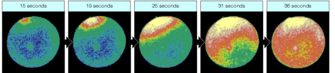
As a first application of the concept of generalised travelling waves of Chapter 4, in Chapter 5 we study calcium waves on spherical eggs. We assume that the waves depend only on the horizontal angle. When we project the waves on the real line we pass from a reaction diffusion equation with constant coefficients on a curved domain to a reaction-diffusion equation with non-constant coefficients on a 1D Euclidean domain. The two striking features of the travelling waves on the real line are (i) the existence of non-trivial steady-state solutions, and (ii) the travelling wave does not invade the whole domain (as it does in the classical 1D case) but it is blocked by the non-trivial steady-state solution. Therefore, the curvature of the sphere plays a crucial role in the properties of the travelling wave.
Gilkey et al [25] studied calcium waves on the eggs of amphibians, which are pretty spher- ical. They found that the waves seem to be invariant under rotations around the vertical axis, and that the velocity of the waves is bigger on the northern hemisphere than on the southern one.
Murray [49] constructed a classical reaction-diffusion equation on the sphere in order to model these calcium waves. However, he found that the model gave the opposite result, namely that the theoretical velocity is smaller in the northern hemisphere than in the southern one. Therefore, the parabolic equation model was discarded and the research on calcium waves turned towards more complex models (e.g. mechano-chemical models based on both parabolic and hyperbolic equations).
However, we found that the conclusions of Murray seem to be wrong. Projecting the equation on the whole real line and truncating the coefficients in order to avoid the singularity of the north and south poles (which are of both mathematical and biological nature), we reproduced the conclusions of Gilkey et al [25], and as such we find the opposite of Murray’s results [49].
Moreover, we also proved that there are two waves, one travelling from the north to the south pole and the other in the opposite sense, and that these travelling waves eventually block each
other, giving rise to non-trivial solutions to the associated elliptic equation. This is an example of generalised travelling waves on the real line, whose velocity of propagation is not constant.
On the unit sphereS2 ∈R3 we consider the reaction-diffusion equation
∂tu−∆S2u=f(u), (0.17)
where ∆S2 denotes the Laplace-Beltrami operator ands7→f(s) is a bistable nonlinearity, i.e.
• f(0) = 0 and f′(0)<0.
• f(1) = 0 and f′(1)<0.
• There exists α ∈ (0,1) such that f(α) = 0, f′(α) > 0, f(s) < 0 for any s ∈ (0, α) and f(s)>0 for anys∈(α,1).
If we restrict our analysis to the class of solutions that are independent of the horizontal angle φthen (0.17) takes the form
∂tu−∂θθu−cotθ ∂θu=f(u), (t, θ)∈R×(0, π). (0.18) Under the change of variablesx= cotθ we obtain an equation on the whole real line,
∂tu−(1 +x2)2∂xxu−x(1 +x2)∂xu=f(u), (t, x)∈R2. (0.19) Notice that the north and south poles (±∞, resp.) are mathematical and biological singularities.
Mathematical singularities because the parametrisation is not bijective on the poles and the coefficients explode, and biological singularities because the underlying biochemical mechanism that triggers the calcium waves is still unknown. Therefore, we will restrict our analysis to a truncated version of (0.19), i.e.
∂tu−a(x)∂xxu−b(x)∂xu=f(u), (t, x)∈R2, (0.20) where
a(x) =
(1 +x2)2 if|x| ≤ρ, (1 +ρ2)2 if|x| ≥ρ, b(x) =
−ρ(1 +ρ2) ifx <−ρ, x(1 +x2) if|x| ≤ρ, ρ(1 +ρ2) ifx > ρ.
For the truncated model (0.20) we have the following four results.
Proposition 0.19 Let (ϕ, c0) be the unique solution of ϕ′′−c0ϕ′+f(ϕ) = 0, lim
z→−∞ϕ(z) = 0, lim
z→+∞ϕ(z) = 1. (0.21)
ϕN :=ϕ
x+cNt 1 +ρ2
, cN = (c0+ρ)(1 +ρ2) for the equation on the north pole, i.e.
∂tu−(1 +ρ2)2∂xxu−ρ(1 +ρ2)∂xu=f(u). (0.22) 2. There is a unique (up to translation) travelling wave solution
ϕS :=ϕ
x+cSt 1 +ρ2
, cS= (c0−ρ)(1 +ρ2) for the equation on the south pole, i.e.
∂tu−(1 +ρ2)2∂xxu+ρ(1 +ρ2)∂xu=F(u). (0.23) In particular, cN > cS.
Theorem 0.20 Suppose that f(s) is a bistable Lipschitz nonlinearity and let cN > 0. Then there exists β > 0 such that the reaction-diffusion equation (0.20) has a unique global solution u(t, x) satisfying
0< u(t, x)<1 ∀(t, x)∈R2 and u(t, x)−ϕ
x+cNt 1 +ρ2
=O(eβt) when t→ −∞, uniformly inx∈R.
In particular,
t→−∞lim
u(t, x)−ϕ
x+cNt 1 +ρ2
= 0 uniformly in x∈R.
Furthermore, t7→u(t, x) is non-decreasing, and if the initial condition u0(x) is non-decreasing thenx7→u(t, x) is also non-decreasing.
Theorem 0.21 Let f(s) be a bistable Lipschitz nonlinearity, and suppose that ρ is sufficiently large such that cS <0. Then there exists β >0 such that the reaction-diffusion equation (0.20) has a unique global solution v(t, x) satisfying
0< v(t, x)<1 ∀(t, x)∈R2 and u(t, x)−ϕ
x+cSt 1 +ρ2
=O(eβt) when t→ −∞, uniformly in x∈R.
In particular,
t→−∞lim
u(t, x)−ϕ
x+cSt 1 +ρ2
= 0 uniformly in x∈R.
Furthermore, t7→ v(t, x) is non-increasing, and if the initial condition v0(x) is non-decreasing thenx7→v(t, x) is non-decreasing.
Theorem 0.22 If we define
u∞(x) := lim
t→+∞u(t, x), v∞(x) := lim
t→+∞v(t, x).
thenu∞(x) and v∞(x) are steady-state solutions of (0.20)satisfying
0< u(t, x)≤u∞(x)≤v∞(x)≤v(t, x)<1 ∀(t, x)∈R2.
Chapter 6. Travelling waves on the sphere
Unlike Chapter 5, where we passed from a homogeneous reaction-diffusion equation on a curved domain to a non-homogeneous reaction-diffusion equation on an Euclidean domain, in Chapter 6 we work directly on the sphere and analyse the properties of generalised travelling waves. We consider here a reaction-diffusion equation with bistable nonlinearity on two domains, a trun- cated sphere with non-homogeneous Dirichlet boundary conditions and the whole sphere with no boundary conditions.
On the truncated sphere we prove that (i) if the nonlinearity is strong enough there are non-trivial solutions of the elliptic problem, (ii) there is a nontrivial solution of the parabolic problem that is strictly increasing in time, i.e. a generalised travelling wave, and (iii) the trav- elling wave is blocked by the non-trivial elliptic solution. On the whole sphere we prove that (i) there are non-trivial solutions of the elliptic problem and (ii) depending on the initial conditions, the solution u(t, x) can converge or not to the stable states 0 and 1. In particular, when the solution does not converge to 0 or 1 the wave does not invade the whole sphere, it does not vanish and if it converges then its convergence is non-monotonic.
Our results on both domains are evidence of solutions that do not invade the whole domain.
Whether there is invasion or not depends on the geometry of the sphere, the strength of the nonlinearity (measured in terms ofλ) and the initial conditions.
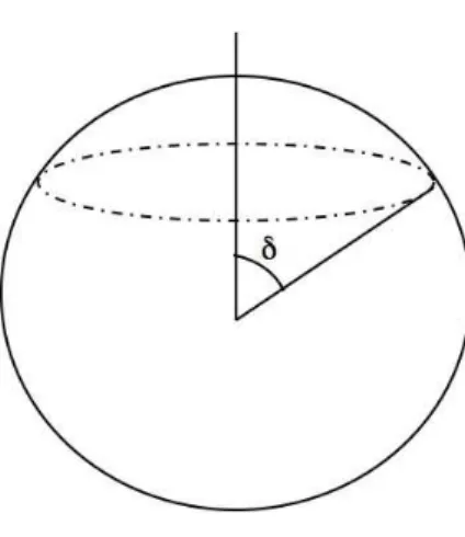
Travelling waves on the truncated sphere Letδ ∈(0, π). We define the truncated sphere as
M={x= (θ, ϕ)∈S2: δ≤θ≤π , 0≤ϕ <2π}, ∂M={θ=δ},
i.e. M is the sphere minus a symmetrical neighbourhood of the north pole of vertical angle δ >0. On Mwe will study the nonlinear elliptic equation
−∆u=λf(u) onM,
u= 1 on ∂M, (0.24)
whereλ >0 and f is bistable, i.e.
• f(0) = 0 and f′(0)<0.
• There exists α ∈ (0,1) such that f(α) = 0, f′(α) > 0, f(s) < 0 for any s ∈ (0, α) and f(s)>0 for anys∈(α,1).
• We extendf onR\[0,1] in aCB1 fashion. More precisely, we will assume that there exist β1 <0 andβ2>1 such that :
– f(s)≡0 fors∈R\(β1, β2).
– f(s)>0 fors∈(β1,0].
– f(s)<0 fors∈(1, β2].
Equation (0.24) is the Euler-Lagrange equation of the functional Jλ(u) = 1
2 Z
M|∇u|2dx−λ Z
M
F(u)dx , F(z) :=
Z z
0
f(s)ds , (0.25) defined on
{u∈H1(M) : u= 1 on ∂M}. It is worth to notice thatF(0) = 0,
F(1) = Z 1
0
f(s)ds and the only constant solution of (0.24) on [0,1] is u≡1.
In order to have a problem defined on H01(M) we use the following change of variables:
w:= 1−u , g(s) :=−f(1−s). Under this framework, equation (0.24) becomes
−∆w=λg(w) onM,
w= 0 on∂M, (0.26)
where g is bistable and share the same properties of f, except that its zero on (0,1) is 1−α.
The associated functional is Iλ(w) = 1
2 Z
M|∇w|2dx−λ Z
M
G(w)dx , G(z) :=
Z z
0
g(s)ds . (0.27) Notice that G(0) = 0, G(1) =−F(1) and the only constant solution of (0.26) on [0,1] isu≡0.
If the non-linearity is too weak, i.e. if the parameter λ >0 is small enough, we prove that the only solution of (0.26) is the trivial solutionw≡0.
Theorem 0.23 There existsλ >0such that for anyλ < λthe only solution of (0.26)isw≡0.
Moreover, if the nonlinearity g(s) does not have the good orientation, that is if its integral on [0,1] is non-positive, then w≡0 is a global minimum.
Theorem 0.24 If G(1)≤0 and λ >0 then w≡0 is the unique global minimum of (0.27).
If the non-linearity is strong enough, i.e. if λ >0 is sufficiently big, we show that we have non-trivial solutions of (0.26).
Theorem 0.25 If G(1)>0 there exists λ♯ >0 such that for any λ > λ♯ we have at least one non-trivial solution of (0.26).
Theorem 0.25 is proven using variational techniques, but using topological techniques e.g.
degree theory we can prove that we have at least two different, non-trivial solutions of the elliptic problem (0.26). Therefore, the non-trivial solutions of (0.26) come in pairs.
Theorem 0.26 If G(1)>0then for any λ > λ♭we have a pair of distinct, non-trivial solutions of (0.26).
Theorem 0.27 Let λ♭ andλ♯ be as in Theorems 0.25 and 0.26, respectively. Then λ♭ =λ♯. From Theorems 0.25 - 0.27 it follows that λ♭ is a pitchfork bifurcation point for the elliptic problem (0.26) because, if there exists one non-trivial solution then there is a second, different non-trivial solution. More precisely, choosing
λ♭= inf{λ >0 : (0.26) has a non-trivial solution}
then for λ < λ♭ the only solution is w ≡ 0 whilst for λ > λ♭ we have two distinct, non-trivial solutions.
Having proven the existence of a non-trivial solution of the elliptic problem (0.26), we can now prove that there is a time-increasing solution of
∂tu= ∆u+λf(u) in (0,∞)× M, u= 1 on (0,∞)×∂M, u(0, x) = 0 for allx∈ M,
(0.28)
i.e. a generalised travelling wave, and that this wave is blocked by the non-trivial solution.
Theorem 0.28 There is a non-trivial solution u(t, x) of (0.28) such thatt7→u(t, x) is strictly increasing, 0< u(t, x)≤u⋆(x) for allt >0 and
t→∞lim u(t, x)≤u⋆(x) ∀x∈ M.
Consider the elliptic nonlinear equation
−∆u=λf(u) on SN ⊂RN+1. (0.29)
wheref ∈C1(R) is the same bistable nonlinearity as in the truncated sphere model. As before, we define
F(z) :=
Z z
0
f(s)ds . The first result is the same as before:
Theorem 0.29 There exists λ > 0 such that for any λ < λ the only solutions of (6.18) are constant.
Definition 0.5 Let u be a solution of (6.18). We say that u is stable if Z
SN
|∇w|2−λf′(u)w2 dx≥0 ∀w∈H1(SN). (0.30)
Property (6.22) is equivalent to say that the first eigenvalueµ1(u) of the operator w7→ −∆w−λf′(u)w
satisfiesµ1(u)≥0.
Theorem 0.30 Let u be a solution of (0.29). If u is stable then it is constant.
From Theorem 0.30, ifu is a non-trivial solution of (6.18) thenu is necessarily unstable and {x∈SN : f′(u(x))>0 } 6=∅.
Theorem 0.30 has been proven by Casten and Holland [12] and Matano [46] in the case of an Euclidean convex domain with homogeneous Neumann boundary conditions. As far as we know, Theorem 6.8 is a new result on manifolds.
Theorem 0.31 There exists λ♭ >0 such that for any λ > λ♭ we have at least one non-trivial solution u⋆(x) of (6.18)such that 0< u⋆ <1.
We have proved that on the whole sphereSN there existsλ∗(=λ) such that for anyλ∈(0, λ∗) the only solutions of (6.18) are constant, and that there exists λ∗(= λ♭) such that for any λ∈(λ∗,∞) there is a non-trivial solutions of (6.18). We conjecture thatλ∗ =λ∗ and that this is true for any compact, connected, smooth manifold without boundary.
Conjecture 0.32 Let M be a compact, connected, smooth manifold without boundary. Then λ∗(M) =λ∗(M), i.e.
• There is bifurcation on the elliptic nonlinear eigenvalue problem
−∆Mu=λf(u) starting at (λ, u) = (λ∗,0),
• for anyλ < λ∗ the only solutions are trivial (i.e. constant), and
• for anyλ > λ∗ we have non-trivial solutions.
In the following chapter we prove Conjecture 0.32 whenM=S1and for a bifurcation starting at the trivial solutionu≡α. However, the general case of a compact, connected, smooth manifold Mwithout boundary is an open problem.
We will show that, depending on the initial conditions, the solution u(t, x) can converge or not to 0 or 1. In particular, when the solution does not converge to 0 or 1 we have that (i) this solution cannot invade the whole sphere, (ii) it does not vanish, and (iii) if it converges then its convergence is non-monotonic.
For anyp∈(0, π) define
A(p) :={x= (ϕ, θ)∈SN : 0≤ϕ <2π, 0≤θ < p}. Letu(p, t, x) be a solution of the problem
∂tu= ∆u+λf(u) in (0,∞)×SN,
u(p,0, x) = 0 for all x∈SN, (0.31) where
u0(p, x) =
1 ifx∈A(p),
0 ifx∈SN\A(p). (0.32)
Theorem 0.33 1. Ifp∼0 then
t→∞lim u(p, t, x) = 0. 2. If p∼π then
t→∞lim u(p, t, x) = 1.
3. There existsp˜∈(0, π)such thatu(˜p, t, x)does not converge to0or1. Ifu(˜p, t, x)converges to a (necessarily untable) solution then its convergence is non-monotonic.
As a final result, we found that the case of a monostable nonlinearity f is much simpler compared to the bistable case. Indeed, not only we always have invasion but also the global solution just depends on time, i.e. it is independent of the space variables.
Denotet7→ξ(t) the unique solution of
ξ′(t) =f(ξ(t)), 0< ξ(t)<1 for allt∈R and ξ(0) = 1 2.
The function ξ is increasing and ξ(−∞) = 0, ξ(+∞) = 1. Let M be a connected compact smooth manifold without boundary (e.g. SN) and denot