[PENDING] Reliability-aware energy optimization for throughput-constrained applications on MPSoC

HAL Id: hal-01766763

https://hal.inria.fr/hal-01766763v1

Submitted on 14 Apr 2018 (v1), last revised 17 Apr 2018 (v2)

HAL is a multi-disciplinary open access archive for the deposit and dissemination of sci- entific research documents, whether they are pub- lished or not. The documents may come from teaching and research institutions in France or abroad, or from public or private research centers.

L’archive ouverte pluridisciplinaire HAL, est destinée au dépôt et à la diffusion de documents scientifiques de niveau recherche, publiés ou non, émanant des établissements d’enseignement et de recherche français ou étrangers, des laboratoires publics ou privés.

Changjiang Gou, Anne Benoit, Mingsong Chen, Loris Marchal, Tongquan Wei

To cite this version:

Changjiang Gou, Anne Benoit, Mingsong Chen, Loris Marchal, Tongquan Wei. Reliability-aware energy optimization for throughput-constrained applications on MPSoC. [Research Report] RR-9168, Laboratoire LIP, École Normale Supérieure de Lyon & CNRS & Inria, France; Shanghai Key Lab.

of Trustworthy Computing, East China Normal University, China; Georgia Institute of Technology, USA. 2018. �hal-01766763v1�

0249-6399ISRNINRIA/RR--9168--FR+ENG

RESEARCH REPORT N° 9168

April 2018

optimization for

throughput-constrained applications on MPSoC

Changjiang Gou, Anne Benoit, Mingsong Chen, Loris Marchal, Tongquan Wei

RESEARCH CENTRE GRENOBLE – RHÔNE-ALPES Inovallée

655 avenue de l’Europe Montbonnot

for throughput-constrained applications on MPSoC

Changjiang Gou

, Anne Benoit

, Mingsong Chen

, Loris Marchal

, Tongquan Wei

Project-Team ROMA

Research Report n° 9168 — April 2018 — ?? pages

Abstract: Multi-Processor System-on-Chip (MPSoC) has emerged as a promising embedded architecture to meet the increasing performance demand of embedded applica- tions. However, due to limited energy budget, it is hard to guarantee that applications on MPSoC can be accomplished on time with a required throughput. The situation becomes even worse for applications with high reliability requirements, since extra energy will be inevitably consumed by task re-executions or duplicated tasks. Based on Dynamic Volt- age and Frequency Scaling (DVFS) and task duplication techniques, this paper presents a novel energy-efficient scheduling model, which aims at minimizing the overall energy con- sumption of MPSoC applications under both throughput and reliability constraints. The problem is shown to be NP-complete, and several polynomial-time heuristics are proposed to tackle this problem. Comprehensive simulations on both synthetic and real applica- tion graphs show that our proposed heuristics can meet all the given constraints, while reducing the energy consumption.

Key-words: Scheduling, MPSoC, energy minimization, throughput, reliability.

∗Laboratoire LIP, ´Ecole Normale Sup´erieure de Lyon & CNRS & Inria, France

†Shanghai Key Lab. of Trustworthy Computing, East China Normal University, China

‡ Georgia Institute of Technology, USA

fiabilit´ e et de d´ ebit

R´esum´e : Le syst`eme multiprocesseur sur puce (MPSoC) est une architec- ture prometteuse pour r´epondre `a la demande de performance croissante des applications embarqu´ees. Cependant, en raison de leur budget ´energ´etique limit´e, il est difficile de garantir que les applications sur MPSoC peuvent ˆ

etre accomplies `a temps avec un d´ebit requis. La situation devient encore pire pour les applications pr´esentant des exigences de fiabilit´e ´elev´ees, car une

´

energie suppl´ementaire sera in´evitablement consomm´ee par des r´e-ex´ecutions de tˆaches ou des tˆaches dupliqu´ees. Bas´e sur le DVFS (Dynamic Voltage and Frequency Scaling) et la duplication de tˆaches, cet article pr´esente un nouveau mod`ele d’ordonnancement, qui vise `a minimiser la consommation d’´energie globale des applications MPSoC sous des contraintes de d´ebit et de fiabilit´e. Le probl`eme est montr´e NP-complet, et plusieurs heuristiques en temps polynomial sont propos´ees pour r´esoudre ce probl`eme. Des simulations compl`etes sur des graphes d’application tant synth´etiques que r´eels montrent que nos heuristiques peuvent r´epondre `a toutes les contraintes donn´ees, tout en r´eduisant la consommation d’´energie.

Mots-cl´es : Ordonnancement, MPSoC, consommation ´energ´etique, d´ebit, fiabilit´e.

1 Introduction

Many smart applications in areas such as Internet of Things (IoT), aug- mented reality, and robotics, increasingly require high performance on em- bedded processing platforms. The three main criteria are i) computational performance, expressed as the throughput of the application; ii) reliability, i.e., most data sets must be successfully computed; and iii) energy efficiency.

This is mainly because: i) some applications such as audio/video coding or deep learning-based inference are delay-sensitive, hence throughput should be properly guaranteed; ii) emerging safety-critical applications such as self- driving vehicles and tactile internet impose extremely stringent reliability requirements [?]; and iii) devices on which smart applications are running are often battery-operated, hence systems should be energy-efficient.

In order to meet all these design constraints, MPSoC is becoming a new paradigm that enables effective and efficient design of smart applications.

By integrating multiple cores together with an interconnection fabric (e.g., Network-on-Chip) as communication backbone, MPSoC (e.g., OMPA from Texas Instruments and NORMADIC from STMicroelectronics) can be tai- lored as multiple application-specific processors with high throughputs but low energy consumption [?, ?].

As one of the most effective power management techniques, Dynamic voltage and frequency scaling (DVFS) has been widely used by modern MP- SoCs [?]. By properly lowering the processing voltages and frequencies of dedicatedly mapped tasks, DVFS enables smart applications to be carried out with a reduced energy consumption, while ensuring a given through- put. However, scaling down voltages and frequencies of processors generates serious reliability problems. Various phenomena such as high energy cos- mic particles and cosmic rays may cause the change of binary values held by transistors within CMOS processors by mistake, resulting in notorious transient faults (i.e., soft errors). Along with the increasing number of tran- sistors integrated on a chip according to Moore’s Law, the susceptibility of MPSoC to transient faults will increase by several orders of magnitude [?].

In other words, the probability of incorrect computation or system crashes will become higher due to soft errors.

To mitigate the impact of soft errors, checkpointing and task replication techniques have been widely used to ensure system reliability [?, ?]. Tasks can be replicated if they do not have an internal state, this increases their reliability as it is extremely unlikely to have errors on two or more copies.

Although checkpointing and task replication techniques are promising on enhancing the system reliability, frequent utilization of such fault-tolerance mechanisms is very time or resource consuming, which will in turn cost ex-

tra energy and degrade the system throughput. Clearly, the MPSoC design objectives (i.e., energy, reliability and throughput) are three contradictory requirements when we need to decide the voltage and frequency level assign- ments for tasks. Although there exist dozens of approaches that can effec- tively handle the trade-off between energy and reliability issues, few of them consider the throughput requirement in addition, see Section ??. Hence, given throughput and reliability constraints, how to achieve a fault-tolerant schedule that minimizes the energy consumption for a specific DVFS en- abled MPSoC platform is becoming a major challenge for designers of smart applications.

To address the above problem, this paper proposes a novel scheduling approach that can generate energy-efficient and soft error resilient mappings for smart applications on a given MPSoC platform. It makes following three major contributions:

1. We propose a novel model that can formally express both performance and reliability constraints for mapping applications on MPSoCs, by bounding the expected period (for performance) and the probability of exceeding the target expected period (for reliability).

2. We prove that without performance and reliability constraints, the problem is polynomially tractable, whereas adding both constraints results in an NP-complete problem.

3. We design and evaluate novel task scheduling heuristics for reliability- aware energy optimization on MPSoCs, which enforce the constraints and aim at minimizing the energy cosumption.

The reminder of this paper is organized as follows. Related work is dis- cussed in Section??. Then, we formalize the application model and optimiza- tion problem in Section??. Section??studies the complexity of the problem variants, and in particular proves that the complete version of the problem is NP-complete. To quickly achieve efficient mappings, Section ?? presents the details of our heuristic approaches. Section ??conducts the evaluation of our approaches on both real and synthetic applications. Finally, Section ??

concludes and provides directions for future work.

2 Related work

MPSoCs have been deployed in various embedded applications such as image processing, process control, and autonomous navigations. Typical MPSoC such as AsAp2 [?] consists of many identical processors with independent

clock domains. They are especially designed for embedded multimedia ap- plications, and featured as high energy efficiency and performance and easy to program [?]. Throughput maximization problem has been a subject of continuing interest as the demands for MPSoC-enabled high performance computing drastically increase. Zhang et al. [?] optimized the throughput in disruption tolerant networks via distributed workload dissemination, and designed a centralized polynomial-time dissemination algorithm based on the shortest delay tree. Li et al. [?] specifically considered stochastic characteris- tics of task execution time to tradeoff between schedule length (i.e., through- put) and energy consumption. A novel Monte Carlo based task scheduling is developed to maximize the expected throughput without incurring a pro- hibitively high time overhead [?]. Albers et al. [?] introduced an online algorithm to further maximize throughput with parallel schedules. However, reliability issues are not considered in these works.

Reliability can be achieved by reserving some CPU time for re-executing faulty tasks due to soft errors [?]. In [?], the authors present a represen- tative set of techniques that map embedded applications onto multicore ar- chitectures. These techniques focus on optimizing performance, temperature distribution, reliability and fault tolerance for various models. Dongarra et al. [?] studied the problem of scheduling task graphs on a set of heterogeneous resources to maximize reliability and throughput, and proposed a through- put/reliability tradeoff strategy. Wang et al. [?] proposed replication-based scheduling for maximizing system reliability. The proposed algorithm incor- porates task communication into system reliability and maximizes communi- cation reliability by searching all optimal reliability communication paths for current tasks. These works explore the reliability of heterogeneous multicore processors from various aspects, and present efficient reliability improvement schemes, however, these works do not investigate the energy consumed by MPSoCs, which interplays with system reliability.

Extensive research effort has been devoted to reduce energy consumption of DVFS-enabled heterogeneous multi-core platforms considering system re- liability. Zhang et al. [?] proposed a novel genetic algorithm based approach to improve system reliability in addition to energy savings for scheduling workflows in heterogeneous multicore systems. In [?], Spasic et al. pre- sented a novel polynomial-time energy minimization mapping approach for synchronous dataflow graphs. They used task replication to achieve load- balancing on homogeneous processors, which enables processors to run at a lower frequency and consume less energy. In [?], Das et al. proposed a ge- netic algorithm to improve the reliability of DVFS-based MPSoC platforms while fulfilling the energy budget and the performance constraint. However, their task mapping approach tries to minimize core aging together with the

susceptibility to transient errors. In [?], the authors considered the problem of achieving a given reliability target for a set of periodic real-time tasks running on a multicore system with minimum energy consumption. The proposed framework explicitly takes into account the coverage factor of the fault detection techniques and the negative impact of DVFS on the rate of transient faults leading to soft errors. Although above works explore various techniques to save energy, to the best of our knowledge, none of the above works considers system throughput in addition to reliability and energy. Our approach is thus the first attempt to model both reliability, performance and energy for workflow scheduling in MPSoC.

3 Model

We consider the problem of scheduling a pipelined workflow onto a homoge- neous multi-core platform that is subject to failures. The goal is to minimize the expected energy consumption for executing a single dataset, given some constraints on the expected and worst-case throughput of the workflow. In the following subsections, we detail how to model applications, platforms, failures, energy cost, period (which is the inverse of the throughput), and how to formally define the optimization problem.

3.1 Applications

We focus on linear chain workflow applications, where task dependencies form a linear chain: each task requests an input from the previous task, and delivers an output to the next task. There are n tasks T₁, . . . , T_n. Further- more, the application is pipelined, i.e., datasets continuously enter through the first task, and several datasets can be processed concurrently by the different tasks. Such applications are ubiquitous in processing of streaming datasets in the context of embedded systems [?].

We assume that the initial data resides in memory, and the final data stays in memory. Task T_j is characterized by a workloadw_j, and the size of its output file to the next tasko_j, as illustrated in Fig.??(except for the last task). In the example, we have w₁ = 2, w₂ = 5,w₃ = 4, and o₁ = 3, o₂ = 1.

Once the first dataset reaches task T₃, while it is processed by T₃, dataset 2 is transferred between T₂ and T₃, dataset 3 is processed by T₂, dataset 4 is transferred betweenT₁ and T₂, and dataset 5 is processed by T₂. At the next period, all dataset numbers are incremented by one.

oj−1 o_j o_j+1 wj wj+1

0 3 1 0

2 5 4

T₁ T₂ T₃

Figure 1: Linear chain workflow application.

3.2 Platforms

The target platforms are embedded systems composed of p homogeneous computing cores. Each core can run at a different speed with a corresponding error rate and an energy consumption. If task T_j is executed on a core operating at speed s(j) and if it is not subject to a failure, it takes a time

wj

s(j) to execute a single dataset.

We focus on the most widely used speed model, thediscretemodel, where cores have a discrete number of predefined speeds, which correspond to dif- ferent voltages at which the core can be operating. Switching is not allowed during the execution of a given task, but two different executions of a task can be executed at different speeds. The set of speeds is {s_min =s₁, s₂, . . . , s_K = s_max}. The continuous model is used mainly for theoretical studies, and let the speed take any value between the minimum speedsmin and the maximum speed s_max.

All cores are fully interconnected by a network on chip (NoC). The band- width β is the same between any two cores, hence it takes ^o_β^j for task Tj to communicate a dataset to task T_j+1. The network on chip enables cores to communicate simultaneously with others while they are computing, i.e., com- munications and computations can be overlapped. Therefore, while task Tj

is processing dataset k, it is receiving the input for dataset k −1 from the previous task, and sending the output for dataset k + 1 to the next task.

Hence, these operations overlap, and take respectively a time ^oj−1_β and ^o_β^j. We follow the model of [?,?], where cores are equipped with a router, and on which there are registers. We can use the registers to store intermediate datasets, hence having buffers between cores. If datasets are already stored in the input buffer of a core, and if there is empty space in the output buffer, then the core can process a dataset without having to wait for the previous or next core.

3.3 Failure model and duplication

Embedded system platforms are subject to failures, and in particular tran- sient errors caused by radiation. When subject to such errors, the system can return to a safe state and repeat the computation afterwards. Accord- ing to the work of [?], radiation-induced transient failures follow a Poisson distribution. The fault rate is given by:

λ(s) = λ₀e^d

smax−s smax−smin,

wheres∈[s_min, s_max] denotes the running speed,dis a constant that indicates the sensitivity to dynamic voltage and frequency scaling, andλ₀is the average failure rate at speed smax. λ0 is usually very small, of the order of 10⁻⁵ per hour [?]. Therefore, we can assume that there are no failures when running at speed s_max. We can see that a very small decrease of speed leads to an exponential increase of failure rate.

The failure probability of executing task T_j (without duplication) on a processor running at speed s_k is therefore f_j(s_k) = λ(s_k)^w_s^j

k. If an error strikes, we resume the execution by reading the dataset again from local memory (i.e., the input has been copied before executing the task, we re- execute the task on the copy), and this re-execution is done at maximum speed so that no further error will strike the same dataset on this task. We assume that the time to prepare re-execution is negligible. Still, this slows down the whole workflow since other tasks may need to wait.

We propose to duplicate some tasks to mitigate the effect of failures and have a reliable execution. This means that two identical copies of a same task are executed on two distinct cores, both core running at the same speed.

In this case, if a failure occurs in only one copy, we can keep going with the successful copy. However, it may increase the energy cost and communication cost. Similarly to one execution at the maximum speed, we assume that an error on a duplicated task is very unlikely (i.e., at least one copy will be successful), and hence f_j(s_k) = 0 if T_j is duplicated.

Let m_j = 1 if task T_j is duplicated, and m_j = 0 otherwise. Let s_k be the speed at which Tj is processed. The failure probability forTj is therefore f_j(s_k) = (1−m_j)λ(s_k)^w_s^j

k, i.e., it is zero if the task is duplicated, and λ(s_k)^w_s^j

k

otherwise (the instantaneous error rate at speed sk times the time to execute task T_j).

If we do not account for communications, the expected execution time of task Tj running at speed sk is:

tj = w_j

s_k +fj(sk) w_j s_max.

Indeed, with duplication, at least one execution will be successful, while with

p_i p⁰_i

p_i+1

p⁰_i+1 p⁰_i

p_i

p_i+1 p_i

p⁰_i

p_i+1

p⁰_i+1 p⁰_i

p_i

p_i+1 p_i

p⁰_i+1

p_i+1 Figure 2: Communications with task duplication.

a single execution, if there is a failure, we re-execute the task at maximum speed and there are no further failures.

If a task is duplicated, this implies that further communications may be done, but they will occur in parallel. If T_j is duplicated, both processors pj and p⁰_j on which Tj is executed are synchronized, and only one of them obtaining a correct result will do the output communication (to one or two processors, depending on whether T_j+1 is duplicated or not), see Fig. ?? for different possible configurations. The synchronization cost is assumed to be negligible.

3.4 Energy

We follow a classical energy model, see for instance [?], where the dissipated power for running at speed s_k is s³_k, and hence the energy consumed for a single execution of task T_j running at speeds_k is ^w_s^j

k ×s³_k=w_js²_k. We further account for possible failures and duplication, hence obtaining the expected energy consumption for T_j running at speed s_k for one dataset:

Ej(sk) = (mj + 1)wjs²_k+fj(sk)wjs²_max.

Indeed, if task T_j is duplicated (m_j = 1), we always pay for two exe- cutions (2wjs²_k) but there is no energy consumed following a failure, while without duplication (m_j = 0), we account for the energy consumed by the re-execution in case of a failure.

We assume that the energy consumed by communications and buffers is negligible compared to the energy consumed by computations, see [?]. There- fore, the expected energy consumption of the whole workflow to compute a single dataset is the sum of the expected energy consumption of all tasks.

3.5 Period definition and constraints

As stated before, each task is mapped onto a different processor, or a pair of processors when duplicated, and different tasks are processing different datasets. In steady-state mode, the throughput is either constrained by the task with the longest execution time, or by the longest communication time,

which is slowing down the whole workflow. The time required between the execution of two consecutive datasets corresponds to this bottleneck time and is called the period. It is the inverse of the throughput.

In this work, we are given a target period P_t, hence the target through- put is _P¹

t. This corresponds for instance to the rate at which datasets are produced. We consider two different constraints: i) ensure that the expected period is not exceeding P_t, hence the target becomes a bound, and/or ii) ensure that the probability of exceeding the target P_t for a given dataset is not greater than proba_t. This second constraint corresponds to real-time systems, where a dataset is lost if its execution exceeds the target periodP_t, and the probability proba_t (0≤ proba_t ≤ 1) expresses how many losses are tolerated. If proba_t = 1, there is no constraint, while proba_t = 0 means that no losses are tolerated.

Recall that the objective is to minimize the expected energy consumption per dataset of the whole workflow. Some tasks may be duplicated, and each task may run at a different speed. The communication between two consecutive tasksT_j and T_j+1 takes a constant time ^o_β^j, and it must fit within the target period. Therefore, we assume that for all 1 ≤j < n, ^o_β^j ≤P_t.

We assume in this section that the set of duplicated tasks is know: we setm_i to 0 or 1 for each taskT_i. Furthermore, let s(i) be the speed at which task T_i is executed, for 1≤i≤n.

We first consider the case without failures and express the period in this case (Section??). Then, we express the expected period when the platform is subject to failures in Section??. Note that we assume that there is a sufficient number of buffers between cores, so that a failure does not necessarily impact the period, given that the cores have access to datasets stored in buffers, and can use empty buffers to store output datasets. Finally, we explain in Section?? how to compute the probability that a dataset exceeds the target period P_t.

3.5.1 Period without failures

In the case without failures, the period is determined by the bottleneck task computation or communication: P_nf= max_1≤i≤nn

wi

s(i),^o_βⁱo .

We denote byLthe set of tasks whose execution time is equal toP_nf, i.e., L=

n

Ti|_s(i)^wi =Pnf

o

. If the bottleneck time Pnf is achieved by a communica- tion, this set may be empty.

3.5.2 Expected period

We consider that each processor is equipped with three or more buffers, two of them holding an input (resp. output) dataset being received (resp. sent), and the other buffers are used for storing intermediate datasets: a buffer is filled when the task is completed, but the following processor is not yet ready to receive the next dataset (i.e., the output buffer is still in use). We consider the period in steady-state, after the initialization has been done, i.e., all processors are currently working on some datasets.

The set of tasksLis empty if the computation time for all tasks is strictly smaller than the periodP_nf. When subject to a failure, tasks not inLcan use data stored in buffers and process datasets at a faster pace than the period, until they have caught up with the time lost due to the failure.

However, errors in tasks of L are impacting the period, and therefore, if such a task is subject to failure, the re-execution time is added to the period.

The expected period can therefore be expressed as follows:

P_exp =P_nf+X

j∈L

f_j(s(j)) w_j

s_max. (1)

Indeed, the period P_nf is achieved when there is either no failure, or a failure in a task not in L. In case of a failure while executing a task Tj inL, the period is P_nf + _s^wj

max, and this happens with a probability f_j(s(j)). As discussed before, we assume that there is no failure during re-execution, and that the probability of having two failures while executing a single dataset is negligible.

Note that this formula also holds when some tasks are duplicated. If task j ∈L is duplicated (mj = 1), it will never fail and hence its period will be P_nf. In this case, f_j(s(j)) = 0 by definition, hence the formula remains correct.

3.5.3 Bounding the probability of exceeding the period bound For the second constraint, we focus on the actual period of each dataset, rather than the expected period, and we estimate the probability at which the period of a dataset exceeds P_t. We consider that P_nf ≤P_t, otherwise the bound can never be reached, and the probability is always one.

The actual period, denoted byP_act, is a random variable that ranges from P_nf to max1≤i≤n

wi

s(i)+ _s^wi

max

. We define the set of tasks that may exceed the target period P_t in case of failures:

S_excess=

T_i | w_i

s(i) + w_i

s_max > P_t

.

Therefore, if a failure strikes a task inS_excesson a given dataset, the target period P_t may not be met for this dataset. An error happens on taski with probability f_i(s(i)). Since failures are independent, the period of a dataset will not exceed the bound if and only if no task in the setS_excesshas a failure, i.e., this happens with a probability Q

Ti∈Sexcess(1−f_i(s(i))).

Hence, the probability of exceeding the bound is given by:

P(P_act> P_t) = 1− Y

Ti∈Sexcess

(1−f_i(s(i)))≈ X

Ti∈Sexcess

f_i(s(i)), (2) considering that the failure probabilities are small, and thatf_i(s(i))×f_j(s(j)) = 0 for any 1 ≤ i, j ≤ n. This approximation is in line with the assumption that we do not consider two consecutive failures in a same task.

Finally, the second constraint that we consider, after the one on the ex- pected period described above, is to bound the probability of exceeding the target period P_t by the target probability proba_t:

P(Pact > Pt)≤proba_t.

3.6 Optimization problems

The objective is to minimize the expected energy consumption per dataset of the whole workflow, and we consider two constraints. The goal is to decide which tasks to duplicate, and at which speed to operate each task. More formally, the problem is defined as follows:

(MinEnergy). Given a linear chain composed of n tasks, a computing plat- form withphomogeneous cores that can be operated with a speed within setS, a failure rate functionf, and a target periodP_t, the goal is to decide, for each task T_j, whether to duplicate it or not (set m_j = 0 or m_j = 1), and at which speed to operate it (choose s(j) ∈ S), so that the total expected energy con- sumption is minimized, under the following constraints:

i) The expected period P_exp should not exceed P_t;

ii) The probability of exceeding the target period P_t should not exceed the target probability proba_t.

Note that if there is a task k such that P_t < _s^wk

max orP_t < ^o_β^k, then there is no solution since the target period can never be met.

If P_t is large enough, the problem will not be constrained since in all solutions, the expected period will always be under the target period. This is the case for P_t ≥ max(_s^wi

min + _s^wi

max) and P_t ≥ max(^o_β^k). In this case, each task running at the slowest possible speed, and being re-executed after a failure, will not exceed P_t. This problem without constraints is denoted as MinEnergy-NoC.

We also consider the particular cases where only one or the other con- straint matters. MinEnergy-PerC is the problem where we do only con- sider the first constraint on the expected period (i.e., set proba_t = 1), while MinEnergy-ProbaC is the problem where we do only focus on the prob- ability of exceeding the target period, i.e., we do not consider P_exp.

4 Complexity analysis

4.1 Without errors

When the workflow is free of errors, a task T_j running at speed s_j takes exactly a time ^w_s^j

j, and consumes an energy of wjs²_j. Hence, to minimize the energy consumption, one must use the smallest possible speed such that the target period is not exceeded, hence s_j = maxn_w

j

Pt, s_mino

in the continuous case. Since we consider discrete speeds, the optimal speed for task Tj is therefore the smallest speed larger than or equal to ^w_P^j

t within the set of possible speeds. This is true for all tasks, hence the problem can be solved in polynomial time.

4.2 Without constraints

We consider theMinEnergy-NoC problem, and propose theBestEnergy algorithm to optimally solve this problem. The idea is to use the speed that minimizes the energy consumption for each task, since we do not have any constraint about exceeding the target period. For each task, either we execute it at this optimal speed, or it may be even better (in terms of energy consumption) to duplicate it and run it at the smallest possible speed s_min. Theorem 1. MinEnergy-NoC can be solved in polynomial time, using the BestEnergy algorithm, both for the discrete and for the continuous energy model.

Proof. Given a task of weightwexecuted at speedswithout duplication, the energy consumption isE(s) = w×s²+λ0w²s²_max^e

d smax−s smax−smin

s . The (continuous) speed that minimizes this energy consumption can be obtained by deriving E(s):

E⁰(s) = 2ws−

λ₀w²s²_max

s² + λ₀dw²s²_max s(s_max−s_min)

e^d

smax−s smax−smin.

E⁰(s) is a monotonically increasing function, and we lets^∗ be the speed such that E⁰(s^∗) = 0, hence E(s^∗) is minimum.

If the task is not duplicated, for MinEnergy-NoC-Cont, the optimal speed iss_opt = max{s^∗, s_min}. In the discrete caseMinEnergy-NoC-Disc, s_optis simply the speed that minimizes the energy consumption, hences_opt = argmin_s∈{s

min,...,smax}{E(s)}.

Now, if the task is duplicated, we assume that it will not be subject to error, hence the energy consumption at speed s is 2ws². Therefore, it is minimum when the task is executed at the minimum speed, and the corre- sponding energy consumption is 2ws²_min (both in the discrete and continuous case).

BestEnergyis a greedy algorithm that sets the speed of each task ats_opt (not using duplication), and then greedily assigns remaining processors to tasks that would gain most from being duplicated (if any), see Algorithm??.

It is easy to see that it is optimal, since any other solutions could only have a greater energy consumption.

Algorithm 1 –BestEnergy(n, p)

1: for i= 1 to n do

2: Computes_opt(i) for taskT_i, the speed that minimizes energy consump- tion if Ti is not duplicated;

3: s_i ←s_opt(i), m_i ←0;

4: g_i ←E(s_i)−2w_is²_min (Possible gain in energy ifT_i is duplicated);

5: end for

6: Sort tasks by non-increasing g_i, T_j is the task with max g_i;

7: p_av ←p−n (Number of available processors);

8: while gj >0 and pav >0 do

9: m_j ←1,s_j ←s_min, p_av ←p_av−1;

10: j ← the index of next task in the sorted list;

11: end while

12: return < s_i, m_i >;

4.3 With the probability constraint

We now prove that the decision version of MinEnergy-ProbaC is NP- complete. In the decision version of MinE-Dec, the goal is to find an assignment set of speeds such that the probability of exceeding the target period P_t does not exceed proba_t, and such that the energy consumption does not exceed a given energy threshold E_t. The proof is based on a re- duction from the Partition problem, known to be NP-complete [?]. The idea is to have only two possible speeds, and one must decide at which speed to

operate each task. We set as many processors as tasks, so that no duplication can be done.

Theorem 2. MinE-Decis NP-complete, even when duplicating tasks is not possible.

Proof. We first check thatMinE-Dec is in NP: given a speed for each task, it is easy to verify in polynomial time whether the bounds on the failure probability and on the energy consumption are satisfied.

The proof of completeness is based on a reduction from the Partition problem, known to be NP-complete [?]. We consider an instance I1−Par of 2-partition: given n positive integers a₁, . . . , a_n, does there exist a partition of {1, . . . , n} into two subsetsI₁ andI₂ (I₁∪I₂ ={1, . . . , n}andI₁∩I₂ =∅) such that P

i∈I₁ai =P

i∈I₂ai =S/2, where S =Pn i=1ai?

We let ∆ = maxa_j/mina_j. We build an instance I2−MinE ofMinE-Dec as follows:

• The workflow is made of n tasks, of size w1 = a1, . . . , wn =an, to be processed on p=n cores (no duplication is possible).

• There are only two possible speeds,s_min=s₁ = 1, and s_max=s₂ = 2∆.

• The failure rate function for these speeds is given by f(s1) = 1/S and f(s₂) = 0.

• We set the target period to P_t = min_iw_i, the bound on the probability of exceeding P_t to proba_t = 1/2, and the bound on the energy to E_t = 2∆²(S+ 1) +S/2.

We first assume that there is a solution (I₁, I₂) to instance I1−Par. For the MinE-Decproblem, we set all tasks T_i withi∈I₁ to speeds₁ = 1, and all tasks T_i with i∈I₂ to speed s₂ = 2∆. Given the target period, we check that S_excess =I₁:

• For any task in I₁, we have w_i/s₁+w_i/s_max> w_i ≥minw_j =P_t.

• For any task inI₂, we havew_i/s₂+w_i/s_max= 2w_i/(2∆) =w_iminw_j/maxw_i ≤ minwj =Pt.

Thus, the probability of exceeding P_t is given by X

i∈I₁

f(s₁)w_i/s₁ = 1/SX

i∈I₁

w_i = 1/S×S/2 = 1/2 =proba_t,

which satisfies the constraint on the probability. Then, we compute the energy of the obtained solution:

E = X

i∈I₁

(w_is²₁+f(s₁)w_is²_max) +X

i∈I₂

w_is²₂

= S/2(1 + 4∆²/S) +S/2·4∆² =E_t,

which satisfies the bound on the energy. Hence, we have found a solution to I2−MinE.

We then assume that I2−MinE has a solution. We denote by I₁ the set of tasks running at speed s₁, and by I₂ the others, running at speed s₂. As outlined below, only tasks in I₁ contribute to the probability of exceeding P_t, and its bound writes:

X

i∈I1

f(s₁)w_i/s₁ ≤1/2 With s₁ = 1 and f(s₁) = 1/S, this gives P

i∈I₁w_i ≤S/2. The bound on the energy writes:

X

i∈I₁

(w_is²₁+f(s₁)w_is²_max) +X

i∈I₂

w_is²₂ ≤ 2∆²(S+ 1) +S/2 X

i

w_is²₁ +X

i∈I1

w_i/Ss²_max+X

i∈I2

w_i(s²₂−s²₁) ≤ 2∆²(S+ 1) +S/2 S+X

i∈I1

w_i/Ss²_max+X

i∈I2

w_i(4∆²−1) ≤ 2∆²(S+ 1) +S/2

X

i∈I2

w_i(4∆²−1) ≤ 2∆²(S+ 1)−S/2−X

i∈I1

w_i/Ss²_max X

i∈I₂

w_i(4∆²−1) ≤ 2∆²(S+ 1)−S/2 X

i∈I₂

w_i(4∆²−1) ≤ S/2(4∆²−1) + 2∆² X

i∈I2

w_i ≤ S/2 + 2∆² 4∆²−1

Since 2∆²/(4∆² −1) < 1 as soon as ∆ ≥ 1 and all w_i’s are integers, this gives P

i∈I2w_i ≤ S/2. Together with P

i∈I1 ≤S/2, this proves that I₁, I₂ is a solution to I1−Par, which concludes the proof.

5 Heuristics

We provide here several heuristics, all designed for the more realistic case of discrete speeds. Heuristics adapted for the case of continuous speeds are presented in Appendix ??. We start with basic heuristics that will be used as baseline. Then we design heuristics aiming at bounding the expected period, and finally heuristics for bounding the probability of exceeding the target period.

5.1 Baseline heuristics

We first outline the baseline heuristics that will serve as a comparison point, but may not satisfy the constraints. First, the BestEnergy algorithm de- scribed in Section?? is providing a lower bound on the energy consumption, but since it means that many tasks are running at the minimum speed, we expect the period to be large, and it may well exceed the bound.

Another simple solution consists in having each task executed at the maximum speed s_max. We refer to this heuristic as MaxSpeed (see Algo- rithm ??).

Algorithm 2 –MaxSpeed(n, p)

1: for i= 1 to n do

2: s_i ←s_max,m_i ←0;

3: end for

4: return < s_i, m_i >;

The third baseline heuristic, DuplicateAll (see Algorithm ??), dupli- cates all tasks, assuming that there are twice more processors than tasks (p ≥ 2n), and the corresponding speeds for each tasks used in this case are Algorithm 3 –DuplicateAll(n, p)

1: if p≥2n then

2: for i= 1 to n do

3: choose s_i as the smallest possible speed so that ^w_sⁱ

i ≤P_t;

4: m_i ←1;

5: end for

6: return < s_i, m_i >;

7: else

8: return failure;

9: end if

the ones derived in Section ??. Indeed, there will not be any errors in this case, and we aim at respecting the target period P_t.

Note that both MaxSpeed and DuplicateAll will always satisfy the bounds, since there will be no errors, and hence the expected period is equal to the period without failure. However, both heuristics may lead to a large waste of energy. They provide an upper bound on the energy consumption when using a naive approach.

5.2 Bounding the expected period

In this section, we focus on the constraint on the expected period, hence targeting the MinEnergy-PerC problem.

5.2.1 Heuristic Threshold

The Threshold heuristic aims at reaching the target expected period P_t (see Algorithm ??). The first step consists in setting all task speeds to the smallest speed such that ^w_sⁱ

i ≤ P_t. If P_exp is still larger than P_t, then one of the tasks with largest duration (^w_sⁱ

i) is duplicated: this allows P_nf to be smaller than P_t and constant from this moment on. Note that in the special case of a communication time reaching P_t, there is no need to duplicate a task to have P_nf =P_t.

From Equation (??),P_exp =P_nf+P

j∈Lf_j(s(j))_s^wj

max. We made sure that P_nf is smaller than or equal to P_t. In order to make P_exp ≤ P_t, each task T_i of L has to be either run at a higher speed (which removes it from L), or duplicated (which sets f_(s(i)) to 0). We greedily duplicate tasks for which duplication costs less energy, until there remains no more processors. Then, we speed up other tasks. Finally, we use the same technique as in BestEn- ergy to attempt to reduce again the energy of non-duplicated tasks: if the minimum speed s for energy consumption is larger than the actual speed s_i of a task T_i, its speed is increased to s.

Algorithm 4 –Threshold(n, p)

1: for all tasks T_i do

2: s_i ← the smallest speed such that ^w_sⁱ

i ≤P_t, m_i ←0;

3: end for

4: p_av ←p−n (number of available processors);

5: if P_t >max(^o_β^k) and p_av ≥1 then

6: Select a taskT_k with largest duration (break tie by selecting one with smallestw_k), set m_k←1 and p_av ←p_av−1;

7: end if

8: if P_exp > P_t then

9: Q← {tasks ofL with m_i = 0};

10: for all tasksTj in Qdo

11: s ←the smallest speed that is larger than s_j;

12: g_j ← w_j ∗(s² +f_j(s)s²_max − 2s²_j) (Possible gain in energy if T_j is duplicated);

13: end for

14: Sort tasks ofQ by non-increasing g_i;

15: for all taskTj in Qdo

16: if p_av >0 then

17: m_j ←1,p_av ←p_av−1;

18: else

19: s_j ←the smallest speed that is larger than s_j;

20: end if

21: end for

22: end if

23: for all task T_i with m_i = 0 do

24: Compute the speeds that minimizes Ei(s);

25: if s_i < sthen

26: s_i ←s;

27: end if

28: end for

29: return < s_i, m_i >;

5.2.2 Heuristic Closer

The previous Threshold heuristic uses duplication: at least one task is duplicated (in order to fix P_nf), which requires spare processors. We propose another heuristic that does not have this requirement. In theCloserheuristic (see Algorithm ??), after setting all task speeds to the smallest ones so that

wi

si ≤ P_t, we increase the speed of all tasks in L while P_exp > P_t by scaling

all tasks simultaneously: we set a coefficient and make sure that for each task, its speed is not smaller than coef ×s⁰_i, where s⁰_i is the initial speed of T_i. The coefficient is gradually increased untilP_exp ≤P_t. Finally, we use the same technique as in BestEnergy to attempt to further reduce the energy consumption of tasks.

Algorithm 5 Closer(n, p,∆s)

1: for all tasks T_i do

2: s⁰_i ← the smallest speed such that ^w_sⁱ

i ≤P_t, m_i ←0;

3: end for

4: Set coef ←1;

5: while P_exp > P_t do

6: coef ←coef + ∆s;

7: for all tasksT_i of setL do

8: s_i ←the smallest speed that is not smaller than coef ×s⁰_i;

9: end for

10: end while

11: for all task T_i do

12: Compute the speeds that minimizes Ei(s);

13: if s_i < sthen

14: s_i ←s;

15: end if

16: end for

17: return < s_i, m_i >

5.3 Bounding the probability of exceeding P

In this section, we design a heuristic focusing on the constraint on the prob- ability of exceeding P_t, thus for the MinEnergy-ProbaCproblem.

BestTrade(see Algorithm??) aims at finding the best tradeoff between energy consumption and the probability of exceeding P_t. We consider for each task two critical speeds:

• sⁱ_c is the speed such that w_i/sⁱ_c+w_i/s_max = P_t; it corresponds to the minimum speed that a task can take without belonging to the S_excess set;

• sⁱ_d = w_i/P_t is the minimum speed that can be assigned to a task: if it is set to a smaller speed, its duration will always exceed the target period.

The idea of the algorithm is first to set all tasks to the smallest speeds that are not smaller than theirsⁱ_cspeed. For some tasks, this might be equal to their minimum speed (the smallest possible speed not smaller than sⁱ_d).

In this case, there is no room for reducing speed again without exceeding the target period. For other tasks, we sort them by non-increasing weight:

tasks with higher weights contribute the most to the energy dissipation and are thus first slowed down: we select the task T_i with the largest weight, reduce its speed to the minimum possible speed not smaller than w_i/P_t. We continue with the tasks of smaller weight, until P(P_act > P_t) ≥ proba_t. At last, if P(P_act > P_t) > proba_t, we just undo the last move to make P(P_act > P_t)<proba_t.

We then consider duplication: if duplicating a task T_i (and setting its speed to the smallest speed that is not smaller thansⁱ_d) is beneficial compared to the current solution (and if a processor is available), the task is duplicated.

Algorithm 6 BestTrade(n, p)

We assume all weights are different (w_i 6=w_j for i6=j);

for j = 1 to j =n do

sj ←smallest possible speed not smaller thanwj/(Pt−w_j/smax),mj = 0;

end for

S_reduce ← tasks that have possible speeds between w_j/P_t and w_j/(P_t − wj/smax);

sort tasks of S_reduce by non-increasing weight;

k = 1;

while P(Pact> Pt)<proba_t do

Reduce speed of k-th task in S_reduce to the smallest that is not smaller than w_j/P_t;

k =k+ 1;

end while

if P(P_act > P_t)>proba_t then

set speed of (k-1)-th task in Sreduce to the smallest that is not smaller than w_j/(P_t−w_j/s_max);

end if

pav ←p−n (Number of available processors);

for j = 1 to j =n do

s_d ← the smallest speed that is not smaller thanw_j/P_t; if 2wjs²_d< wjs²_j +fj(sj)wjs²_max and pav >0 then

duplicate T_j, m_j = 1, s_j =s_d, p_av ←p_av−1;

end if end for

6 Experimental validation through simulations

In this section, we evaluate all proposed algorithms through extensive sim- ulations on both real applications and synthetic ones, in the case of dis- crete speeds. Results with continuous speeds are available in Appendix ??.

For reproducibility purposes, the code is available at https://github.com/

gouchangjiang/Pipeline_on_MPSoC.

Given a computing platform and an application, we set the target period P_tand probabilityproba_t so that all assumptions made in the model are true:

• When all tasks are executed with the minimum speed smin, the max- imum failure rate is not larger than 10⁻². With such a failure rate, the failure of two copies of a duplicated task is very unlikely, and the approximation in Equation (??) holds.

• When all tasks are processed with speed s_max, the maximum failure rate is not larger than 10⁻⁴, which means that the failure of a task running at maximum speed is very unlikely.

• Ptshould not be smaller than any task duration when running at max- imum speed, otherwise, there is no way to meet the target period:

P_t≥ ^max(w_s ⁱ⁾

max .

We setPt =a+κ∗(b−a), wherea= max(wi/smax, oi) andb=max(wi/smin+ w_i/s_max, o_i): a(respectivelyb) is the maximal time spent on a task (either on computation or on communication), when running at the maximum (resp.

minimum) speed. This way, Pt is never smaller than a, which satisfies the third condition above. Similarly, we avoid the case P_t ≥ b, in which the target is too loose, as even the minimum speed can achieve it. A small κ leads to a tighter target period. Under the above three conditions, we set κ to values from 0.05 to 0.95, by increment of 0.01. The target probability is set to proba_t = 0.05 for synthetic applications and proba_t = 0.01 for real applications.

We use the result of heuristic BestEnergy described in Section ?? as a comparison basis, as it gives the minimum energy consumption of the system without any constraint.

6.1 Multi-core embedded systems

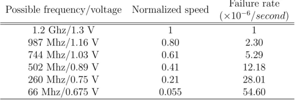
We simulate a multi-core computing platform with 512 cores. Based on AsAP2 and KiloCore, two state-of-art MPSoCs described in Section ??, the frequency/voltage options are listed in Table ??. NoC on chips enables ex- tremely fast communications. We describe the value of β together with the

output (input) file sizes o_i below in the next subsection. The failure rate is computed as described in Section ?? as λ(s) = λ₀e^d

smax−s

smax−smin. Based on the settings in [?], we set λ₀ = 10⁻⁶ and d= 4.

Possible frequency/voltage Normalized speed Failure rate (×10⁻⁶/second)

1.2 Ghz/1.3 V 1 1

987 Mhz/1.16 V 0.80 2.30

744 Mhz/1.03 V 0.61 5.29

502 Mhz/0.89 V 0.41 12.18

260 Mhz/0.75 V 0.21 28.01

66 Mhz/0.675 V 0.055 54.60

Table 1: Configurations of computing platforms.

6.2 Streaming applications

We use a benchmark proposed in [?] for testing the StreamIt compiler. It collects many applications from varied representative domains, such as video processing, audio processing and signal processing. The stream graphs in this benchmark are mostly parametrized, i.e., graphs with different lengths and shapes can be obtained by varying the parameters. Table??lists some linear chain applications (or application whose major part is a linear chain) from [?].

Some applications, such as time-delay equalization, are more computation intensive than others.

Following the same idea, we also generated synthetic applications in order to test the algorithms on larger applications. We generated 100 groups of linear chains. Each group contains 3,000 linear chains with the same number of nodes, which range from 0.01p to pfrom group to group by an increment 0.01p, where p is the number of cores. The weights of the nodes w_i follow a truncated normal distribution with mean value 2,000, where the values smaller than 100 or larger than 4,000 are removed. The standard deviation is 500. This ensures that the execution time is not too long so that failure rate is acceptable. The communication time (^o_βⁱ) follows a truncated normal distribution with mean value 0.001∗Pt, values that are larger than Pt are replaced by P_t. Here P_t =a+ 0.05∗(b−a).

6.3 Simulation result

We present both results on synthetic applications and on real applications.

On each plot, we show the minimum, mean, and maximum values of each

Application Size Average node’s weight

CRC encoder 46 14.20

N-point FFT (coarse-grained) 13 1621.31 Frequency hopping radio 16 11815.81

16x oversampler 10 2157.4

Radix sort 13 179.92

Raytracer (rudimentary skeleton) 5 142.8 Time-delay equalization 27 23264.78

Insertion sort 6 475.83

Table 2: Real application examples.

heuristic. In some cases, only the mean is plotted to ease readability, when the minimum and maximum do not bring any meaningful information.

6.3.1 Synthetic applications

0 20 40 60

0.25 0.50 0.75

κ

Expected Period

Heuristics BestEnergy BestTrade Closer DuplicateAll MaxSpeed Threshold

(a) Expected period

0.000 0.025 0.050 0.075 0.100

0.25 0.50 0.75 κ

Probability of exceeding the period bound

(b) Probability

0 10 20 30 40

0.25 0.50 0.75

κ

Energy cost normalized to BestEnergy

(c) Energy consumption Figure 3: Energy consumption and constraints on synthetic applications, as a function of κ.

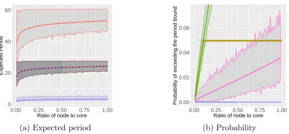
Fig. ?? presents the results of all heuristics, both in terms of energy consumption, and in terms of constraints, when we vary the parameter κ, hence the tightness of the bound on the expected period. On Fig. ??, the dashed lines represent the minimum, maximum and average period bound.

All chains have 0.5p nodes. Apart from MaxSpeed, which always meets the bound, and BestEnergy, which never meets the bound, all heuristics succeed to meet the bound on the expected period. BestTrade,Closerand DuplicateAll are overlapped byThreshold.

Fig. ?? shows the probability of exceeding the period bound, and the dashed line is the targetproba_t. DuplicateAllis overlapped byMaxSpeed, and only BestTrade succeeds to always meet the bound. Closer and