HAL Id: hal-00856672
https://hal.archives-ouvertes.fr/hal-00856672v4
Submitted on 11 Mar 2015
HAL is a multi-disciplinary open access archive for the deposit and dissemination of sci- entific research documents, whether they are pub- lished or not. The documents may come from teaching and research institutions in France or abroad, or from public or private research centers.
L’archive ouverte pluridisciplinaire HAL, est destinée au dépôt et à la diffusion de documents scientifiques de niveau recherche, publiés ou non, émanant des établissements d’enseignement et de recherche français ou étrangers, des laboratoires publics ou privés.
Weak second order multi-revolution composition methods for highly oscillatory stochastic differential
equations with additive or multiplicative noise
Gilles Vilmart
To cite this version:
Gilles Vilmart. Weak second order multi-revolution composition methods for highly oscillatory stochastic differential equations with additive or multiplicative noise. SIAM Journal on Scien- tific Computing, Society for Industrial and Applied Mathematics, 2014, 36 (4), pp.1770-1796.
�10.1137/130935331�. �hal-00856672v4�
Weak second order multi-revolution composition methods for highly oscillatory stochastic differential equations
with additive or multiplicative noise
Gilles Vilmart∗ April 15, 2014†
Abstract
We introduce a class of numerical methods for highly oscillatory systems of stochas- tic differential equations with general noncommutative noise. We prove global weak error bounds of order two uniformly with respect to the stiffness of the oscillations, which permits to use large time steps. The approach is based on the micro-macro framework of multi-revolution composition methods recently introduced for determin- istic problems and inherits its geometric features, in particular to design integrators pre- serving exactly quadratic first integral. Numerical experiments, including the stochastic nonlinear Schr¨odinger equation with space-time multiplicative noise, illustrate the per- formance and versatility of the approach.
Keywords: highly-oscillatory stochastic differential equation, composition method, quadratic first integral conservation, multiplicative noise, time-dependent stochastic Schr¨odinger equation.
MSC numbers: 60H10, 35Q55.
1 Introduction
Consider a nonlinear system of (Itˆo1) stochastic differential equations (SDEs) of the form dX(t) = (ε−1AX(t) +f(X(t)))dt+
Xm r=1
gr(X(t))dWr(t), 0≤t≤T, (1) whereε >0 is fixed,A∈Rd×dis a constant matrix, f, gr :Rd→Rd are smooth and Lips- chitz vector fields,X(0) =X0 is the initial condition, andWr, r= 1, . . . , mare independent standard Wiener processes. On the highly oscillatory part of the problem, we assume that
exp(A) =I. (2)
∗Universit´e de Gen`eve, Section de math´ematiques, 2-4 rue du Li`evre, CP 64, 1211 Gen`eve 4, Switzerland.
On leave from ´Ecole Normale Sup´erieure de Rennes, INRIA Rennes, IRMAR, CNRS, UEB, av. Robert Schuman, F-35170 Bruz, France, Gilles.Vilmart@ens-rennes.fr
†A typographical error was corrected in Theorem 3.3 (Dec. 2014).
1We focus on Itˆo SDEs to simplify the presentation, but our analysis applies also to Stratonovich SDEs using the conversion formula.
This means that the flow of the stiff oscillatory partdXdt =ε−1AX, given byx7→exp(ε−1tA)x, is periodic with respect to t, with periodε. Thus, multiple oscillatory frequencies inε−1A are allowed if they are integer multiples of 2π. Such class of problems includes second order SDEs of the form
X(t) =¨ −ε−2K2X(t) +a(X(t)) + Xm r=1
br(X(t)) ˙Wr(t) (3) where K ∈ Rd×d is a constant positive symmetric matrix with eigenvalues in 2πN and a, br :Rd → Rd are smooth vector fields. An interesting situation is the case where a =
−∇U derives from a potential U :Rd→Rand where additive noise is considered, i.e. the functionsgr are constant and there exists a constant matrixB ∈Rd×m such that
(g1(q), . . . , gm(q)) =B. (4)
Consider the Hamiltonian, which represents the energy of the system (3), H(p, q) = 1
2 pTp+ε−2qTK2q+U(q) .
A standard application of the Itˆo formula to (3) yields that the average of Hamiltonian grows linearly with time due to the additive noise perturbation. Precisely, setting Q(t) = X(t) andP(t) = ˙X(t), we have
E(H(P(t), Q(t))) =H(P(0), Q(0)) + t
2trace(BBT) (5)
and this energy is exactly conserved along time only in the deterministic case (B = 0).
The linear growth (5) is not recovered in general by standard explicit integrators, e.g. the Euler-Maruyama method where a super linear growth can be observed [10, 11].
The class of problems (1) also includes spectral spatial discretizations of the nonlinear Schr¨odinger equation with a stochastic space-time noise. Consider for instance
i∂u(x, t)
∂t =−∆u(x, t) +εV(x)|u(x, t)|2qu(x, t) +√
εg(u(x, t)) ˙W(x, t), t≥0, x∈(0,1), (6) where we consider periodic boundary conditions in dimension one of space for simplicity.
Here, W(x, t) denotes a real-valued white noise which is white in time and correlated in space.2 We refer for more details to [15] where numerical simulations of the stochastic Schr¨odinger equation are presented to investigate the influence of space-time noise over the stochastic blow up time of the solutions, and to [13] where the strong and weak convergence rates of the Euler-Maryama method applied to a class of stochastic nonlinear Schr¨odinger equations are shown to be the same as for SDEs in finite dimension (i.e. weak order 1) in contrast to the parabolic case. In the case of multiplicative noise in the Stratonovitch sense where g(u) = σu (with σ a constant), we have that the L2 norm R1
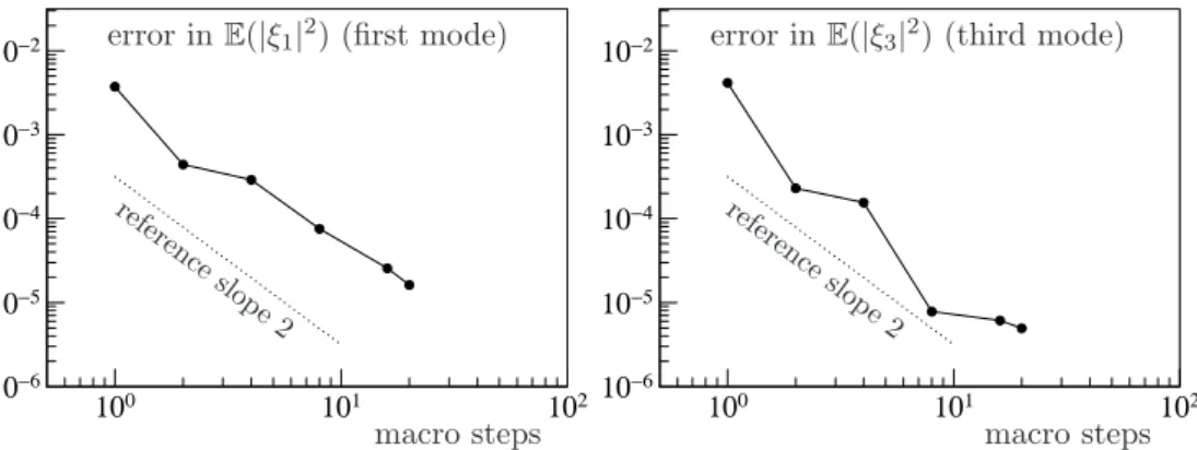
0 |u(x, t)|2dx is a first integral similarly to the deterministic: it is exactly conserved along time almost surely on the existence interval of the solution. The Hamiltonian energy is however not conserved in general in the presence of noise. Considering a pseudo-spectral spatial representation of the form u(t, x) ≈ Pℓ
k=−ℓ+1ξk(t)eikx with a fixed number ℓ of Fourier modes, we then
2Here, the correlation in space arises from the fixed numberℓof Fourier modes considered in the noise.
arrive at the following system of SDEs with Stratonovitch noise for the Fourier modes ξk(t)∈C, −ℓ < k ≤ℓ,
dξk = −ik2ξk+ε fk(. . . , ξ−1, ξ0, ξ1, . . .)
dt+iσ√ ε X
ℓ<j≤ℓ
ξk−j◦dWj, (7) where fk corresponds to the nonlinear term V|u|2qu, Wj (−ℓ < j ≤ ℓ) are independent standard Wiener processes, and we setξj±2ℓ=ξj for alljin the above sum (the convolution product of the solution frequencies and the Wiener processes). The Stratonovitch system of SDEs (7) can be recast into the format (1) by rescaling time (that is, by rewriting the system in terms of the new time variable ˆt = 2πε t) and using the Stratonovitch to Itˆo conversion formula.
For the numerical approximation of highly oscillatory problems of the form (1), standard SDE integrators require in general a time stepsize of the same magnitude as ε to achieve stability and accuracy, which can be prohibitively expansive for small values ofε, already in the deterministic setting (gr = 0, r= 1, . . . , min (1)), and thus appropriate integrators are needed. For the numerical study of highly oscillatory stochastic integrators and not assuming (2), we mention the recent work [34], where splitting methods for the Langevin equations are analyzed, and the works [10, 12] where stochastic trigonometric methods are proposed and analyzed, and further extended to the linear stochastic wave equation [11].
The trigonometric methods are a modification of the classical leap-frog method for (3) where filter functions are introduced to avoid numerical resonances (see [21, Chap. XIII] in the context of deterministic problems). A common aspect of the aforementioned works is the study of the strong convergence (with orders 1/2 or 1), i.e. the errorE(|X(tk)−Xk|) (where tk=kh andh is the stepsize) for approximating individual trajectoriesX(t) themselves in the case of additive noise (i.e. (4) holds). In contrast, we consider here the general case of a general nonlinear noncommutative noise, and we focus on the weak error of convergence, i.e. the error|E(φ(X(tk)))−E(φ(Xk))|where φis a smooth test function.
In [7], the class of deterministic multi-revolution composition methods was recently introduced for systems of the form (1) withgr = 0, r = 1, . . . , m. Observe that the exact flow of this problem after one periodεis a smooth perturbation of the identity. The multi- revolution approach, as first proposed in [23, 27], permits the approximation of the Nth iterate of a smooth deterministic near identity mapϕε(y) =y+O(ε) fromRdinto itself, but calculating only a few compositions (hence the name multi-revolution). SettingH := N ε, a example of such composition method is the order two approximation of theNth iterate of the mapϕε,
ϕ(H+ε)/2◦ϕ−1−(H−ε)/2(y) =ϕNε (y) +O(H3).
It is shown in [7] that the constant symbolized byO is independent ofN ≥1 andε≤ε0 if ϕε(y) is a C3 function of (y, ε). Next, considering for ϕε the flow of an highly oscillatory system after one highly oscillatory period permits to design large time step geometric in- tegrators. The aim of this paper is to extend and analyze this approach to the stochastic context with general nonlinear multi-dimensional drift and diffusion functions.
It is known (see [29] and the recent work [9]) in a deterministic context (gr = 0) that the solutionX(t) of (1) is asymptotically close to an effective nonstiff problem of the form
dX(t)
dt = a1+εa2+ +ε2a3+. . . X(t)
, X(0) =X0 (8)
where a1(x) =
Z 1
0
esAf(e−sAx)ds a2(x) = −1
2 Z 1
0
Z s2
0
es2Af(e(s1−s2)Af(e−s1Ax))−es1Af(e(s2−s1)Af(e−s2Ax))
ds1ds2,
. . . (9)
at times which are integer multiples of the oscillatory period. Precisely, truncating the above series (8) (which diverges for general nonlinear problems) after theεp−1 term yields X(t) = X(t) +O(εp) for all t = kε ≤ T with k ∈ N, and this remainder can be made exponentially small for analytic data. We observe that the vector field of the effective problem (8) involving multiple integrals can be difficult to simulate in general. Although an analogous effective problem can be constructed in some cases (see Remark 3.5 for additive noise), we highlight that the proposed methods do not involve the pre-calculation of such an effective problem but applies directly to the original problem (1), with micro and macro stepsizes in the spirit of the so-called Heterogeneous Multiscale Method [2, 16, 17].
This paper is organized as follows. In Section 2, we introduce the stochastic multi- revolution composition methods and state our main weak convergence results. In Section 3, we perform the error analysis of the proposed methods for general nonlinear systems of SDEs. In Section 4, we present several numerical examples and comparisons with other oscillatory integrators that corroborate the theoretical orders of convergence and illustrate the good qualitative behavior of the proposed methods for various problems over long times, including the stochastic nonlinear Schr¨odinger equation with multiplicative noise.
2 Multi-revolution composition methods for oscillatory SDEs
We first introduce semi-discrete multi-revolution methods involving a macro time stepsize H which can be possibly much larger than the oscillatory periodε. We next introduce the fully-discrete methods by coupling the multi-revolution approach with a micro integrator involving in addition a micro stepsize h. We present weak error estimates with respect to H, hwith error constants independent ofε. The proofs are postponed to Section 3.
2.1 Semi-discrete multi-revolution composition methods
We introduce the following integrator which permits to integrate (1) with oscillatory period εon a time interval of size O(1) at a computational cost independent of ε by considering appropriate auxiliary non-stiff SDE problems.
Algorithm 2.1 (Semi-discrete S-MRCM). For the approximation of the flow after time H=N ε of (1) where N ∈N, we consider the scheme Xk7→Xk+1 defined by
dKk,1 = (−AKk,1+αNHf(Kk,1))dt+p αNH
Xm r=1
gr(Kk,1)dWk,r,1, Kk,1(0) =Xk (10) dKk,2 = (AKk,2+βNHf(Kk,2))dt+p
βNH Xm r=1
gr(Kk,2)dWk,r,2, Kk,2(0) =Kk,1(1) (11) Xk+1=Kk,2(1)
where Wk,r,1, Wk,r,2, r= 1, . . . , m are independent Wiener processes, and we define αN := 1
2 − 1
2N, βN := 1 2 + 1
2N. (12)
For notational brevity, we shall sometimes drop the dependence onkofKk,j andWk,r,j. The advantage of the above Algorithm 2.1 is that the stiff problem (1) on a time interval H = N ε including N fast oscillations (due to the term ε−1AX in (1)) is approached by the resolution of two non-stiff problems posed on the time interval (0,1) involving each only one oscillation, and thus more convenient to solve. In other words, in this multi- revolution approach, N fast oscillations of (1) are approached by only two oscillations of analogous problems with appropriate coefficients. This is advantageous compared to standard integrators for large values ofN, i.e. for small values ofε.
Remark 2.2. In the context of deterministic oscillatory problems, order conditions for MRCMs up to arbitrary high order are derived in [7] using the algebraic framework of la- belled rooted trees, and integrators up to order4are exhibited. However, it is known [30, 31]
that a composition method with real coefficients of order strictly larger than2necessarily in- volves negative coefficients, see [4] for an elegant geometric proof. Since stochastic problems such as (1)are not reversible in time, such high order methods cannot straightforwardly be applied. A possibility to circumvent this order barrier for non-reversible problems would be to use complex coefficients, as proposed in [5, 22] in the context of deterministic diffusion problems. The use of complex coefficients in this context is however beyond the scope of the present paper.
The next task is to prove accuracy estimates between the exact solutionX(t) of (1) and the approximationXk from Algorithm 2.1 wheret=kH andH =N εwith error constants independent ofH ≤H0 and ε≤ε0. We make the following smoothness assumption of the data.
(H) The functionsf,gr, r= 1, . . . , mareC6-functions with all partial derivatives bounded.
This implies that f, gr are Lipschitz continuous (but not necessarily bounded), and thus the solution of (1) exists and is unique. In order to state our weak error estimates, we denote CPp(Rd,R) the set of functions of class Cp where all the partial derivatives have a polynomial growth, i.e. for each partial derivative φup to order p, there exist C >0 and r∈N such that
|φ(x)| ≤C(1 +|x|r). (13) We shall prove in Section 3 the following second order weak error estimate for the semi-discrete methods.
Theorem 2.3. Let T > 0. Assume (2) and (H). Consider Xk the numerical solution of Algorithm 2.1 and X(t) the exact solution of (1). Then, for all φ ∈ CP6(Rd,R), and all H=N ε withN ∈N, and k∈Nwith kH ≤T,
|E(φ(Xk))−E(φ(X(kH)))| ≤CH2, where the constantC is independent of ε, H, k, N.
We highlight that the weak accuracy estimate of Theorem 2.3 holds uniformly with respect toεwhere bothε≪1 andε≃1 are allowed. Observe in addition that Algorithm 2.1 is exact forN = 1 (i.e. the error is zero) becauseKk,1(1) =Xk in (10) and (11) reduces to a time transformation ˆt=t/εof (1).
Remark 2.4. Notice that setting αN = 0, βN = 1 in (12) in the definition of Algorithm 2.1 would yield the following multi-revolution method Xk7→Xk+1 of weak order1,
dKk = (AKk+Hf(Kk))dt+√ H
Xm r=1
gr(Kk)dWk,r, Kk(0) =Xk, Xk+1 =Kk(1).
Indeed, the error estimate of Theorem 2.3 with H2 replaced by H remains valid for the above scheme for allφ∈CP4(Rd,R) (observe in this case Kk,2(0) =Kk,1(1) =Xk). In this paper, we shall however focus on the more accurate weak second order methods. The error analysis of the first order method can be performed analogously.
2.2 Fully-discrete multi-revolution composition methods
Algorithm 2.1 is called semi-discrete because each step requires the resolution of two systems of SDEs, whose solution is not known in general and needs to be approximated numerically.
It was noted in the deterministic context [7] that in principle, any nonstiff integrator could be used. However, a natural choice for such approximation is to use a splitting method where the oscillatory and non oscillatory parts of the problem are solved separately in an efficient way (sometimes exactly), as proposed and studied recently in [34] in the stochastic context of the Langevin equation.
We now formulate the fully-discrete multi-revolution stochastic methods for the class of problems (1). It involves a micro stepsize h and a macro stepsize H where H ≫ ε is allowed. We highlight again that bothH andh are of moderate size, independently of the smallness of the stiff parameterε. The approach involves a weak integratorYk+1 = Φh(Yk) with stepsizeh for the nonstiff SDE problem
dY(t) =f(Y(t))dt+ Xm r=1
gr(Y(t))dWr(t) (14)
where compared to (1), the stiff term ε−1A has been removed. The integrator Φh can be the exact solution if computationally available, or an efficient weak approximation.
Algorithm 2.5(Fully-discrete S-MRCM). Consider a macro stepsizeH =N εand a micro stepsize h = 1/n with N, n ∈N∗. For the approximation of the flow after time H of (1), we consider the scheme Xk+1 7→Xk defined by the composition
Xk+1= (ehA/2◦ΦβNHh◦ehA/2)n◦(e−hA/2◦ΦαNHh◦e−hA/2)n(Xk)
where the micro integrator Φh is a weak integrator for (14) with stepsize h, and αN, βN
are defined in (12). The exponents n indicate that the maps are composed n times with independent random variables.
Notice that Algorithm 2.5 requires for each time step 2n applications of the nonstiff integrator Φh, applied with independent random variables, and 2nevaluations of exponen- tials (usingehA/2◦ehA/2 = ehA). The following theorem with proof postponed to Section 3 states that it has weak second order of accuracy with respect to the micro and macro stepsizesH, h, uniformly with respect to ε. To this aim, we assume that the integrator Φh satisfies for allx∈Rd, and all h≤h0,
|E(Yk+1−Yk|Yk =x)| ≤C(1 +|x|)h, |Yk+1−Yk| ≤Mk(1 +|Yk|)√
h, (15) where C, Mn are independent of h, x and Mk is a random variable with finite moments of all orders. We further assume the following local weak order two estimate, for all φ ∈ CP6(Rd,R),
|E(φ(Φh(Y0)))−E(φ(Y(h)))| ≤C(x)h3, (16) whereC(x) is independenthand has a polynomial growth (13).
Theorem 2.6. Let T > 0. Assume (2) and (H). Consider Xk the numerical solution of Algorithm 2.5 andX(t) the exact solution of (1). Assume that the integrator Φh for (14) satisfies (15) and (16). Then, for all φ∈CP6(Rd,R), and all h = 1/n and H =N εsmall enough with n, N, k∈N withkH ≤T,
|E(φ(Xk))−E(φ(X(kH)))| ≤C(H2+h2), (17) where C is independent ofε, H, n, k, N, h.
The proofs of the above weak convergence estimates (Theorem 2.3 and Theorem 2.6) are provided in Section 3.
Remark 2.7. We highlight that (15) and (16) are natural assumptions for a weak order two integrator. Indeed, a classical theorem of Milstein [24] (see [25, Chap. 2.2]) permits to deduce from the local error (16) the global error |E(φ(Yk))−E(φ(Y(hk)))| ≤ Ch2 for all hk ≤ T. Crucial is the assumption (15), which is easily satisfied by any reasonable integrator for (14), and that automatically yield that Yk has bounded moments of any order for allkh≤T (see [25, Lemma 2.2, p. 102]). Examples of such integrators with additional favorable geometric properties are presented in Section 4.
We end this section with the following remark, which shown that the multi-revolution approach has links with weak methods for systems of SDEs with small noise of the form
dZ(s) =a(Z(s))dt+εb(Z(s))dt+p
|ε| Xm r=1
cr(Z(s))dWr(s), Z(0) =Z0 (18) as proposed and analyzed in [26] (see also [25, Chap. 3]). Such schemes applied to (18) have global weak orderO(hp +εhq) where p < q on bounded time intervals, using appropriate smoothness assumptions on the vector fieldsa, b, cr.
Remark 2.8. Setting a(Z) = AZ, b(Z) = f(Z), σr = gr, Z0 = X0, the system (18) is equivalent to (1) via the time transformation s = t/ε. In this case, the multi-revolution approach permits to approximate Z(s) on longer time intervals with s = O(ε−1) with a computational cost and an accuracy both independent of ε. Indeed, following the lines of the proof of Theorem 2.6, if Ψh,ε is an integrator for (18) with weak order O(hp +
εhq), then, provided the numerical moments remain uniformly bounded, the multi-revolution composition scheme
Xk+1= (Ψh,βNH)n◦(Ψ−h,−αNH)n(Xk),
with αN, βN defined in (12) and h = 1/n, can be shown to approximate the solution X(t) of (1) at time t =kH with H = N ε with global weak error O(H2 +H−1hp+hq) for all kH≤T (equivalently to approximate (18) at time s=kN ≤ε−1T), where the constant in O is independent of H, h, ε.
3 Weak convergence analysis
A crucial ingredient for the analysis is the variation of constant formula: the solutionX(t) of (1) satisfies
X(t) =etε−1AX0+ Z t
0
e(t−s)ε−1Af(X(s))ds+ Z t
0
e(t−s)ε−1A Xm r=1
gr(X(s))dWr(s). (19) In other words, considering the change of variablesY(t) =e−ε−1tAX(t), we have thatY(t) is the solution of the non-autonomous SDE problem
dY(t) =e−ε−1tAf(eε−1tAY(t))dt+ Xm r=1
e−ε−1tAgr(eε−1tAY(t))dWr(t). (20) A feature of the semi-discrete Algorithm 2.1 is that it is exact in the case of additive noise (4) and in the absence of the nonlinearity (f = 0), as stated in the following proposition.
This is a consequence of the homogeneity and scaling in time properties of Wiener processes.
Notice in contrast that the stochastic trigonometric methods [10, 12] are not exact in this case.
Proposition 3.1. Consider the numerical solution of (1)withf = 0and additive noise(4).
Then, Algorithm 2.1 is exact in the sense that X(t), t =kN ε and Xk have the same law of probability for allε and all N, k,∈N.
Proof. The solutions of (10) and (11) can be expressed using the variation of constant formula (19), which yields, usingeA=e−A=I,
X1 =X0+√ H
Z 1
0
e−sABdW˜(s) where we notice that ˜W(s) :=√αNW1(s)+√
βNW2(s) is a standardm-dimensional Wiener process because αN +βN = 1 (recall that W1 and W2 are assumed independent). In comparison, using (19) and the change of variable ˆs=ε−1s, and the periodicity oft7→etA with period 1, the exact solution of (1) withf = 0 and (4) satisfies
X(H) =X0+ Z N
0
e−sABdW(εs) =X0+ Z 1
0
e−sAB
NX−1 k=0
dW(εs+k).
Using standard homogeneity and scaling in time properties of the Wiener process, we have thatH−1PN−1
k=0 (W(εs+k)−W(k)) is also a standard Wiener process. Using the indepen- dence ofWk,1, Wk,2, k= 0,1,2, . . .in Algorithm 2.1, we obtain thatX(H) has the same law of probability as X1, and we conclude the proof that X(tk) and Xk have the same law of
probability by induction onk.
Using (2), we observe that for integer multiples of the oscillatory period, the solutions of (1) and (20) coincide: X(N ε) = Y(N ε) for all N ∈ N and all ε. The advantage of considering the form (20) compared to (1) is that the drift and diffusion functions (x, t)7→
e−ε−1tAf(eε−1tAY(t)) and (x, t) 7→ e−ε−1tAgr(eε−1tAY(t)) are C6-functions with all partial derivatives with respect to the spatial variable x bounded uniformly with respect to ε.
Using these regularity, we may recall the following two classical results taken from [33].
Lemma 3.2. [33, Lemma 1]. Assume (H) and consider the solutionY(t) of (20). Then, there exist a constantC >0 andr ∈N such that for all p∈N, t∈[0, T], X0∈Rd,
E(|X(t)|p)≤C(1 +|X0|r).
In addition, there exists a version of the process X(t) which is almost surely 6 times con- tinuously differentiable with respect to the initial conditionX(0) =X0, and the derivatives with respect to the initial condition, (∂kX(t))/(∂X0k), k = 1, . . . ,6, have bounded moments uniformly with respect to ε∈R, t∈[0, T], X0 ∈Rd.
Theorem 3.3. [33, Theorem 2.2]. Assume (H) and consider the solution Y(t) of (20).
ForT >0 and all φ∈CP6(Rd,R), the function v(x, t) :=E(φ(Y(t))|Y(T) =x), 0≤t≤T, is solution of the Backward Kolmogorov partial differential equation
∂v
∂t +Lε(−t)v= 0, v(x, T) =φ(x), where the generator of (20) is defined by3
Lε(−t)φ(x) = e−ε−1tAf(eε−1tAx)· ∇φ(x)
+ 1
2 Xm r=1
φ′′(x)
e−ε−1tAgr(eε−1tAx), e−ε−1tAgr(eε−1tAx)
(21) and the partial derivatives ∂ti0∂xi1· · ·∂xikv(x, t) with 2i0 +k ≤ 6, 1 ≤ ij ≤ d, i0, k ≥ 0, are continuous with polynomial growth (13) where r, C are independent of ε, x ∈Rd, and t∈[0, T]. In particular,
u(x, t) :=E(φ(Y(t))|Y(0) =x) (22) is equal tov(x, T −t), and assumingT /ε∈Nand (2), we obtain thatu(x, t) in (22)is the solution of
∂u
∂t =Lε(t)u, u(x,0) =φ(x), (23)
for allt∈[0, T].
We deduce from Theorem 3.3 a weak Taylor expansion foru(x, H) =E(φ(X(H))) where X(t) is the solution of (1).
Proposition 3.4. Assume the hypotheses of Theorem 3.3. Then, u(x, t) defined in (22) satisfies for all H=N ε, withN ∈N,
u(x, H) = φ(x) +H Z 1
0 L1(s1)φ(x)ds1+H2−Hε 2
Z 1
0
Z 1
0 L1(s1)L1(s2)φ(x)ds2ds1
3We denote∇φ(x) the gradient with respect toxofφandφ′′(x)(·,·) the second derivative ofφ, which is a symmetric bilinear form.
+ Hε Z 1
0
Z s1
0 L1(s1)L1(s2)φ(x)ds2ds1+O(H3)
where the constant in O(H3) is independent of N, ε with a polynomial growth (13) with respect to x, and L1 is defined in (21) withε= 1.
Proof. Iterating “´a la Picard” the integral relation u(x, t) = φ(x) +Rt
0Lε(s)u(x, s)ds, we obtain
u(x, t) = φ(x) + Z t
0 Lε(s1)φ(x)ds1+ Z t
0
Z s1
0 Lε(s1)Lε(s2)φ(x)ds2ds1 +
Z t 0
Z s1
0
Z s2
0 Lε(s1)Lε(s2)Lε(s3)u(x, s3)ds3ds2ds1
which yields using Theorem 3.3, u(x, H) =φ(x) +
Z H
0 Lε(s1)φ(x)ds1+ Z H
0
Z s1
0 Lε(s1)Lε(s2)φ(x)ds2ds1+O(H3) where the constant in O(H3) satisfies the polynomial growth (13) uniformly with respect toN, ε. Using the change of variable ˆsi =ε−1si, we deduce
u(x, H) =φ(x) +ε Z N
0 L1(s1)φ(x)ds1+ε2 Z N
0
Z s1
0 L1(s1)L1(s2)φ(x)ds2ds1+O(H3).
Finally, using the periodicity assumption (2) yields the identities Z N
0 L1(s1)φ(x)ds1 = N Z 1
0 L1(s1)φ(x)ds1, Z N
0
Z s1
0 L1(s1)L1(s2)φ(x)ds2ds1 = N(N −1) 2
Z 1
0
Z 1
0 L1(s1)L1(s2)φ(x)ds2ds1
+ N
Z 1
0
Z s1
0 L1(s1)L1(s2)φ(x)ds2ds1,
which permits to conclude the proof.
A consequence of Proposition 3.4 is the following remark, which gives some insight on a stochastic effective problem in the case of additive noise, analogously to (8).
Remark 3.5. Consider the additive case (4) with dimensionsd=m and B=I. It can be checked that for alltk=kε≤T withk∈N, and all φ∈CP6(Rd,R),
|E(φ(X(tk)))−E(φ(X(tk)))| ≤Cε2, where C is independent ofN, ε, where X(t) solves the effective SDE
dX =
a1+ε(a2+σ2∆b2)
(X)dt+σ(I+εb′2(X))dW(t), X(0) =X0 (24) where a1, a2 are defined in (9) and
b2(x) = 1 4
Z 1
0
s1es1Af(e−s1Ax)− Z s1
0
es2Af(e−s2Ax)ds2
ds1.
The proof of (24) is deduced showing first the local estimate|E(φ(X(ε)))−E(φ(X(ε)))| ≤ Cε3 (using Proposition 3.4 with N = 1for X(ε) and analogously a weak Taylor expansion forX(ε)). Interestingly, the effective SDE (24)has multiplicative noise in general, although the original SDE (1)with B =I in (4)has additive noise.
We may now derive a local weak error estimate for the semi-discrete S-MRCM.
Lemma 3.6. Assume (2) and (H). Consider X1 the numerical solution of Algorithm 2.1 after one step and X(t) the exact solution of (1). Then, for all initial condition X0 = x, allφ∈CP6(Rd,R), and all H =N εwith N ∈N,
|E(φ(X1))−E(φ(X(H)))| ≤C(x)H3,
where the constantC(x) is independent of ε, H and has a polynomial growth (13).
Proof. We observe that the SDE (10) has the form (1) by settingε=−1 and replacingf byαNHf and gr by√
αNHgr. Applying Proposition 3.4 withN = 1, we deduce E(φ(K1(1))|K1(0) =x) = φ(x) +αNH
Z 1
0 L−1(s1)φ(x)ds1
+ (αNH)2 Z 1
0
Z s1
0 L−1(s1)L−1(s2)φ(x)ds2ds1+O(H3). (25) Analogously for the solution K2(t) of (11), we have
E(φ(K2(1))|K2(0) =x) = φ(x) +βNH Z 1
0 L1(s1)φ(x)ds1 + (βNH)2
Z 1
0
Z s1
0 L1(s1)L1(s2)φ(x)ds2ds1+O(H3), (26) where the constants in the above remainders O(H3) are independent of N, ε and have a polynomial growth (13) with respect tox.
We next have by the Fubini theorem and using properties of conditional expectancies (recall thatW1, W2 in (10),(11) are independent Wiener processes),
E(φ(X1)|X0 =x) =EW1
EW2
φ(K2(1))|K2(0) =K1(1)
|K1(0) =x
(27) where the notationsEW1,EW2 refers to the expectation with respect to the Wiener process W1, W2, respectively. Applying (25) with φ replaced by x = K2(0) 7→ EW2(φ(K2(1))), which is, by Theorem 3.3, almost surely of classC6 with derivatives of polynomial growth, we deduce for allX0=xthe estimate4
E(φ(X1)) =
I+αNH Z 1
0 L−1(s1)ds1+ (αNH)2 Z 1
0
Z s1
0 L−1(s1)L−1(s2)ds2ds1
◦
I+βNH Z 1
0L1(s1)ds1+ (βNH)2 Z 1
0
Z s1
0 L1(s1)L1(s2)ds2ds1
φ(x) +O(H3)
4Observe that the ordering of composition is the opposite compared to the ordering (10),(11) in Algorithm 2.5. This effect is known as the “Vertauschungssatz” of Gr¨obner in the deterministic literature, see e.g. [21, Sect. III.5.1].
=
I+αNH Z 1
0 L−1(s1)ds1+βNH Z 1
0 L1(s1)ds1
+ αNβNH2 Z 1
0 L−1(s1)ds1
Z 1
0 L1(s1)ds1
+ (αNH)2 Z 1
0
Z s1
0 L−1(s1)L−1(s2)ds2ds1 + (βNH)2
Z 1
0
Z s1
0 L1(s1)L1(s2)ds2ds1
φ(x) +O(H3).
A consequence of (2) isR1
0 L−1(s1)ds1 =R1
0 L1(s1)ds1 and Z 1
0
Z s1
0 L−1(s1)L−1(s2)ds2ds1 = Z 1
0
Z 1
0 L1(s1)L1(s2)ds2ds1− Z 1
0
Z s1
0 L1(s1)L1(s2)ds2ds1. We deduce
E(φ(X1)) =
I + (αN +βN)H Z 1
0 L1(s1)ds1 + (αNβN +α2N)H2
Z 1
0
Z 1
0 L1(s1)L1(s2)ds2ds1 + (βN2 −α2N)H2
Z 1
0
Z s1
0 L1(s1)L1(s2)ds2ds1
φ(X0) +O(H3).
Using (12), we observe that αN +βN = 1, (αNβN +α2N)H2 = (H2−Hε)/2 and (βN2 − α2N)H2 = Hε. Comparing the above Taylor expansion with the one in Proposition 3.4
permits to conclude the proof.
Based on the local error estimate of Lemma 3.6, we may now give the proof of Theorem 2.3 for the global order two of convergence in the weak sense. To this aim, the following lemma, which is shown in the proof of [25, Lemma 2.2, p. 102] is a crucial ingredient.
Lemma 3.7. [25] Consider a discrete process{Yk}(k∈N) satisfying (15). Assume further thatY0 has finite moments of all orders. Then, for all integerp, there existsCp such that
E(|Yk|p)≤eCpkh(E(|Y0|p) + 1) for allk∈N and h≤h0.
Proof of Theorem 2.3. We use a well known result of Milstein [24] (see [25, Chap. 2.2]) which permits to deduce automatically the global error estimate of Theorem 2.3 from the local error estimate of Lemma 3.6. To this aim, we only have to check is that the moments E(|Xk|2r) of the numerical solution are bounded for all k, H with 0 ≤kH ≤T uniformly with respect tokandHsufficiently small. This is a consequence of Lemma 3.7 applied with h=H to the discrete process{Yk}defined byY2k=Xk andY2k+1=Kk,1(1) whereKk,1 is given in (10). Considering the SDEs (10) and (11), the estimates (15) with h=H for the discrete flowsKk,1(0)7→Kk,1(1) andKk,2(0)7→Kk,2(1) are a straightforward consequence of the Lischitzness off, gr, r= 1, . . . , m. This permits to conclude the proof.
In order to prove Theorem 2.6 for the the global weak accuracy of the fully-discrete method, we need to check that the numerical solution has uniformly bounded moments of any order. This is the purpose of the following lemma which shows that the numerical moments are uniformly bounded in spite of the oscillatory terms e±hA/2 involved in the scheme.
Lemma 3.8. Assume the hypotheses of Theorem 2.6 and consider the numerical solution Xk of Algorithm 2.5. Then, for all p ∈ N, there exists a constant Cp such that for all H=N ε, k∈N withkH ≤T,
E(|Xk|p)≤Cp.
Proof. We observe that the numerical solutionXk+1is calculated inductively fromXkusing a composition of 2nstochastic mappings of the form
eδhA/2◦ΦγhH ◦eδhA/2
where δ = −1, γ = αN or δ = 1, γ = βN. Let {Yκ}, κ = 0,1,2, . . . denote the discrete process arising from this composition (note thatXk =Y2nk). We next define the discrete processYeκ fromYκ by
Ye2nk+j =ejhAY2nk+j, Ye2nk+n+j =e−jhAY2nk+n+j, , j= 1, . . . , n.
For 1≤j ≤n, we obtainYe2nk+j+1=eh(j+1/2)A◦ΦαNhH◦e−h(j+1/2)A(Ye2nk+j),which yields Ye2nk+j+1−Ye2nk+j =eh(j+1/2)A(ΦαNhH(e−h(j+1/2)AYe2nk+j)−e−h(j+1/2)AYe2nk+j).
Analogously, for n+ 1 ≤ j ≤ 2n, the above identity holds with A replaced by −A and αN replaced by βN. Using the estimates (15) on Φh, the inequality |eλAξ| ≤ c|ξ| for all λ∈R, ξ ∈Rd, and the bounds αN ≤1, βN ≤1 we deduce for allκ,
|E(Yeκ+1−Yeκ|Yeκ =x)| ≤C(1 +|x|)Hh, |Yeκ+1−Yeκ| ≤Mκ(1 +|Yeκ|)√ Hh, whereC is independent ofN, n, H, h, ε, κ, k. Applying Lemma 3.7 then yields that Yeκ has uniformly bounded moments of any order for κHh ≤ 2T. We conclude the proof using
h= 1/n andXk=Ye2nk for all k.
We shall also need the following result, whose proof follows standard arguments. For the sake of completeness, a proof is provided in Appendix.
Lemma 3.9. Assume the hypotheses of Theorem 2.6. Let δ = −1, γ = αN (resp. δ = 1, γ=βN). Then, the integrator
Yk+1=eδhA/2◦ΦγHh◦eδhA/2(Yk),
applied the SDE (10) (respectively (11)) satisfies for allφ∈CP6(Rd,R) and all H, h= 1/n small enough,
|E(φ(Yn))−E(φ(Kj(1)))| ≤C(x)h2H,
where j= 1 (resp. j= 2) and C(x) is independent of h, H, N, n, k, ε and satisfies (13).
Proof of Theorem 2.6. Consider the numerical solution denoted ˆXk of the semi-discrete Algorithm 2.1. Applying Lemma 3.9 for (10) and (11), we deduce
|E(φ( ˆX1))−E(φ(X1))| ≤C(x)h2H.
Using Lemma 3.6, we deduce the local error estimate
|E(φ(X1))−E(φ(X(H)))| ≤C(x)(H3+h2H). (28) In addition, by Lemma 3.8, the numerical solution Xk as uniformly bounded moments of any order, and the Milstein theorem [24] (see [25, Chap. 2.2]) then yields the global error
estimate of Theorem 2.6.
4 Numerical experiments
In this final section, we consider four problems to illustrate numerically the weak conver- gence rates of the proposed methods and the versatility of the approach. We investigate not only the accuracy of the methods compared to other oscillatory integrators but also their long time qualitative behavior. We also compare our approach with other known highly oscillatory integrators.
4.1 An illustrative example: Kubo oscillators
We first focus on the so-called Kubo oscillators. A nonlinear version with multiplicative Stratonovitch noise, as considered recently in [10], is
dQ(t) = (−ε−1P(t) +P f(P(t), Q(t)))dt+σP(t)◦dW(t)
dP(t) = (ε−1Q(t)−Qf(P(t), Q(t)))dt−σQ(t)◦dW(t) (29) whereP(t), Q(t)∈Rand the same one-dimensional Wiener process is considered in (29) for both components. Notice that (29) can be put in the form (1) using the time transformation ˆt=t/2πand the Stratonovitch to Itˆo conversion formula. For the nonstiff part of the system (29), we choose as micro integrator a Strang splitting method
Φh = ΦVh/2◦ΦWh ◦ΦVh/2, (30) where, on the one hand, the noise partdQ=σP ◦dW, dP =−σQ◦dW is integrated with
ΦVh : q
p
7→
Q P
=
cos(σ√
hξ) sin(σ√ hξ)
−sin(σ√
hξ) cos(σ√ hξ)
q p
whereξare independent random variables withP(ξ =±√
3) = 1/6,P(ξ= 0) = 2/3. Notice that replacing above √
hξ by ∆Wk =W((n+ 1)k)−W(nk) would make ΦVh exact. The above choice of discrete random variable makes ΦVh a weak second order integrator (using E(ξ2) = 1,E(ξ4) = 3). On the other hand, the nonlinear part dQ = σP f(P, Q)dt, dP =
−σQf(P, Q)dt is approximated by the implicit midpoint rule defined as ΦWh :
q p
7→
Q P
=
q+hPMf(PM, QM) p−hQMf(PM, QM)
wherePM = (p+P)/2, QM = (q+Q)/2. In the implementation of ΦWh , we use fixed point iterations until convergence up to round-off errors. Notice that the splitting scheme (30) has weak second order of accuracy (see Proposition 6.1 in Appendix withε= 1).
100 101 102 10−5
10−4 10−3 10−2 10−1
100 101 102
10−5 10−4 10−3 10−2 10−1
100 101 102
10−5 10−4 10−3 10−2 10−1
100 101 102
10−5 10−4 10−3 10−2 10−1 semi discrete MRCM (ε= 2−6)
macro steps reference
slope 2
semi discrete MRCM (ε= 2−8)
macro steps reference
slope 2
fully discrete MRCM (ε= 2−6)
macro steps reference
slope 2
fully discrete MRCM (ε= 2−8)
macro steps reference
slope 2
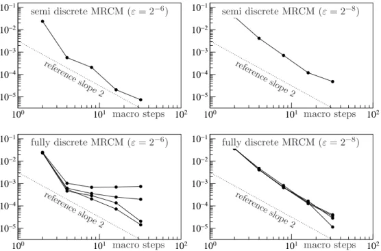
Figure 1: Multi-revolution methods for the Kubo oscillator (29) with nonlinearityf(p, q) = p3+q5. Error inE(Q(T)2) versus number of macro steps (final timeT = 2π). Top pictures:
semi-discrete S-MRCM. Bottom pictures: fully-discrete S-MRCM with n = 8,16,32,64 micro steps per macro step (respectively from top to bottom).
Conservation of quadratic first integrals An interesting feature of (29) is that the quantity C(p, q) = p2 +q2 is exactly conserved along time for all trajectories. Precisely, observing that d C(P(t), Q(t))
= 0 (as shown for instance in [10, Prop. 3.2]), we have almost surely
P(t)2+Q(t)2 =P(0)2+Q(0)2, for all t >0. (31) Since both integrators ΦVh and ΦWh exactly conserve the quadratic first integral, we have that Φh in (30) exactly conserves P(t)2 +Q(t)2, and thus also the corresponding fully- discrete S-MRCM of Algorithm 2.5: Pk2+Q2k = P02+Q20 for all k ∈ N and all numerical trajectories of the method. Note in contrast that the strong method proposed in [10] does not conserve exactly this quadratic first integral in general.
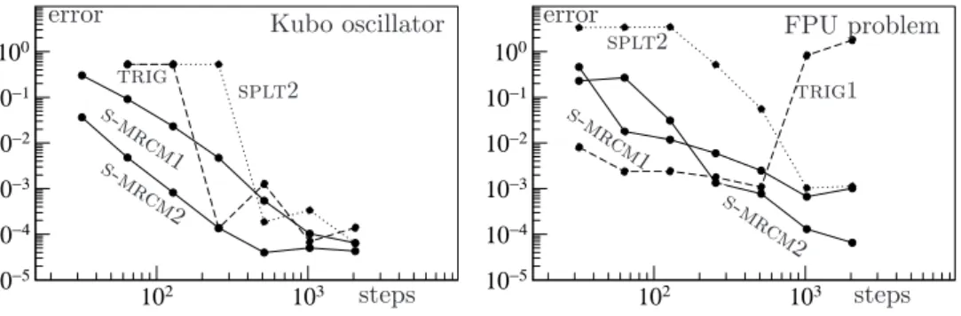
Weak convergence rates Since the scheme exactly conserves the quadratic first integral P2+Q2, we have that the weak error bound (17) holds provided thatf :R2→Rin (29) is of classC6in a neighbourhood of{(p, q) ; p2+q2 =P0+Q0}where we consider a deterministic initial condition (here Q0 = 1, P0 = 0). We consider the nonlinearity f(p, q) = p3 +q5 (similarly to [10]). For ε= 2−6 ≃1.6·10−2 (left pictures) and ε= 2−8 ≃3.9·10−3 (right pictures), we plot for many different macro stepsH the error for the second moment of the first componentE(|Q(T)|2) at the final time T = 2π as a function of the number of macro stepsT /H. The expectation is approximated using the average over M = 107 trajectories to make the Monte-Carlo error sufficiently small compared to the weak accuracy of the methods. In the top pictures, we take n = 1024 micro steps in each macro step, so that the micro discretization can be considered as nearly exact (see semi-discrete Algorithm
2.1). In the bottom pictures, the four lines correspond respectively to n = 8,16,32,64 micro steps per macro step (from top to bottom lines). In the top pictures, we observe the expected lines of slope 2, as proved in the semi-discrete error analysis of Theorem 2.3.
In the bottom pictures, we observe the expected lines of slope 2 only for a sufficiently fine micro stepsize, as shown in Theorem 2.6. As a reference solution, we consider here the standard Strang splitting eε−1hA/2 ◦Φh◦eε−1hA/2 with Φh defined in (30) with small stepsizeh= 2−15T ≃1.9·10−4.
4.2 A test problem with non-commutative noise
In some situations (e.g. the stochastic nonlinear Schr¨odinger model (7) studied in Section 4.4), the exact solution of the non oscillatory system (14) is available and easy to compute.
Otherwise a weak second order approximation is needed in general. Notice that already for nonstiff stochastic problems and without structure assumptions (i.e. for a non-commutative noise), methods with high strong order are generally costly to simulate because they involve multiple stochastic integrals, such as Rh
t0
Rs2
0 dWq(s1)dWr(s2), which are costly to approxi- mate strongly for q 6= r. This is however not true for weak methods where such multiple stochastic integrals can be approximated efficiently in a weak sense using appropriate dis- crete random variables. The aim of this section is to illustrate that this is again not a difficulty in our highly oscillatory context. We consider the following nonlinear oscillatory problem in dimensiond= 2, which is a modification of a scalar test SDE from [14], with a non-commutative Itˆo noise with m= 10 independent driving Wiener processes,
dQ(t) = −ε−1P(t)dt, Q(0) = 1, (32)
dP(t) = ε−1Q(t)dt+ X10
j=1
a−1j q
P(t)2+Q(t)2+b−1j (1−Q(t))dWj(t), P(0) = 0.
where P(t), Q(t) ∈ R. The values of the constants aj, j = 1, . . . ,10 are respectively 5, 5, 10, 15, 30, 15, 10, 5, 10, 15, and the values of bj, j = 1, . . . ,10 are respectively 4, 3, 5, 2, 1, 2, 4, 5, 10, 10. Considering the averaged oscillatory energyE =E P2+Q2
, an application of the Itˆo formula yields dE(t)dt =P10
j=1a−2j (E(t) +b−1j (1−cos(t/ε))),which can be solved analytically as
E P(t)2+Q(t)2
=eat+b(a+a3ε2)−1 eat+a2ε2cos(t/ε)−aεsin(t/ε)−a2ε2−1 , wherea=P10
j=1a−2j = 37/225,b=P10
j=1a−2j b−1j = 257/6000. We shall use this formula to check the accuracy of the fully-discrete S-MRCM (Algorithm 2.5).
For the integratorX1 = Φh(X0) needed to integrate the non-stiff part of problem (32), which has the form (14) with f = 0, we compare two different schemes which fulfil the assumptions of Theorem 2.6. On the one hand we simply use the Euler-Maruyama method of weak order 1,
X1 =X0+√ h
Xm r=1
gr(X0)ξr,
whereξr are independent discrete random variables satisfyingP(ξr=±√
3) = 1/6,P(ξr= 0) = 2/3. On the other hand, we consider the following Runge-Kutta type scheme of weak order two, which is a derivative free version of the Milstein-Talay method [32] derived in