HAL Id: tel-00765238
https://tel.archives-ouvertes.fr/tel-00765238v2
Submitted on 17 Jul 2013
HAL is a multi-disciplinary open access archive for the deposit and dissemination of sci- entific research documents, whether they are pub- lished or not. The documents may come from teaching and research institutions in France or abroad, or from public or private research centers.
L’archive ouverte pluridisciplinaire HAL, est destinée au dépôt et à la diffusion de documents scientifiques de niveau recherche, publiés ou non, émanant des établissements d’enseignement et de recherche français ou étrangers, des laboratoires publics ou privés.
Long Yu Jiang
To cite this version:
Long Yu Jiang. Séparation et détection des trajets dans un guide d’onde en eau peu profonde. Autre.
Université de Grenoble, 2012. Français. �NNT : 2012GRENT050�. �tel-00765238v2�
Sp´ecialit´e: Signal, Image, Parole et T´el´ecom Arrˆet´e minist´eriel :7ao ˆut2006
Present´ ee par´
Longyu JIANG
These dirig` ee par´ J´er ˆome I. Mars
prepar´ ee au sein du´ Laboratoire Gipsa dans l’´Ecole Doctorale:
Electronique Electrotechnique Automatique Traitement du Signal
S´eparation et d´etection de trajets dans un guide d’onde en eau peu profonde
These soutenue publiquement en` 22. Nov. 2012, devant le jury compose de´ :
Monsieur Philippe Roux
DR, ISTERRE, CNRS Grenoble, Pr´esident Monsieur Salah Bourennane
PR, Institut Fresnel, Ecole Centrale de Marseille, Rapporteur Monsieur Jean Pierre Sessarego
DR, LMA, CNRS Marseille, Rapporteur Monsieur Gang Feng
PR, Gipsa-lab, Grenoble-INP, Examinateur Monsieur Herv´e Liebgott
MCF, CREATIS, Universit´e Lyon1, Examinateur Monsieur J´er ˆome I Mars
PR, Gipsa-lab, Grenoble-INP, Directeur de Th`ese
To my parents.
Where there is a will, there is a way.
—-Thomas Alva Edison
I owe my deepest gratitude to Mr. Feng Gang. Without his helps, I would not have obtained the chance of beginning my doctorate study in Gipsa-lab.
I would like to thank the president of my oral defense committee —- Mr. Philippe Roux. He is a world-class scientist and give me useful advices for the future studies.
I wish to thank the two reviewers of my thesis —- Mr. Salah Bourennane and Mr.
Jean Pierre Sessarego. They are the distingushed experts in both signal processing and in underwater acoustics. My thesis is well reviewed by them. These very good comments are encouragements of my research life, even ones of my life.
I am indebted to the members of my oral defense committee —- Mr. Herv´e Liebgott and Mr. Feng Gang. They suggest that I should continue this study in several other applications; for instance, medical application.
It is with immense gratitude that I acknowledge the support and help of my super- visor —- Mr. J´er ˆome I. Mars. Without his guidance and patience this dissertation would not have gone on smoothly.
I am indebted to my many colleagues who supported me a lot, especially Silvia and Franc¸ois. Our discussions about research, cultures, food and daily life made the research life more colorful. Besides, they also give me a lot of encouragements when I faced difficulties in research. These encouragements gave me greater confidence in overcoming difficulties.
I cannot find words to express my gratitude to my friends, especially Shenghong and her husband. They are warm-hearted, sincere and easy-going. They always put themselves in my place, and help me a lot to the best of their abilities.
Finally, I wish to thank my parents, my sister, my brother in law and my new nephew. Their love is a driving force for my advance forever. My dissertation is dedi- cated to them.
5
As the studies on shallow-water acoustics became an active field again, this dissertation focuses on studying the separation and detection of raypaths in the context of shallow- water ocean acoustic tomography. As a first step of our work, we have given a brief review on the existing array processing techniques in underwater acoustics so as to find the difficulties still faced by these methods. Consequently, we made a conclusion that it is still necessary to improve the separation resolution in order to provide more useful information for the inverse step of ocean acoustic tomography. Thus, a survey on high- resolution method is provided to discover the technique which can be extended to sepa- rate the raypaths in our application background. Finally, we proposed a high-resolution method called smoothing-MUSICAL (MUSIC Actif Large band), which combines the spatial-frequency smoothing with MUSICAL algorithm, for efficient separation of co- herent or fully correlated raypaths. However, this method is based on the prior knowl- edge of the number of raypaths. Thus, we introduce an exponential fitting test (EFT) using short-length samples to determine the number of raypaths. These two methods are both applied to synthetic data and real data acquired in a tank at small scale. Their performances are compared with the relevant conventional methods respectively.
Keywords: array processing, shallow water, source separation, ocean acoustic tomogra- phy, smoothing-MUSICAL, exponential fitting test.
7
Acknowledgments 5
Abstract 7
Contents 9
List of Figures 15
List of Tables 19
1 Introduction 1
1.1 Objectives . . . 4
1.2 Outline . . . 5
2 Background knowledge on Ocean Acoustic Tomography 7 2.1 Fundamentals of Ocean Acoustics . . . 10
2.2 Characteristic Sound Paths . . . 12
2.3 Sound Propagation Models . . . 14
2.3.1 Ray Theory . . . 15
2.3.2 Parabolic Equation (PE) Model . . . 16
2.4 General Technique Steps of OAT . . . 18
2.5 OAT in Shallow Water Waveguide . . . 19
2.5.1 Shallow Water . . . 19
2.5.2 Recent Studies on Shallow water . . . 20
2.5.3 Multiple RayPaths Propagation . . . 22
3 Array Processing in Underwater Acoustics 25 3.1 Sampling and Digitization Techniques . . . 27
3.1.1 Plane-Wave Beamforming . . . 27
3.1.2 Adaptive Beamformers (Maximum-likelihood method (MLM)) . . 28
3.1.3 Double Beamforming . . . 29
3.1.4 A Gibbs sampling localization-deconvolution approach . . . 31
3.1.4.1 Signal model in time domain . . . 33 9
3.1.4.2 Gibbs sampler . . . 33
3.2 Directly from the received signals . . . 37
3.2.1 Matched Field Processing . . . 37
3.2.1.1 Green’s functions . . . 37
3.2.1.2 Signal Models . . . 38
3.2.1.3 Noise Models . . . 38
3.2.1.4 Sample covariance estimation . . . 39
3.2.1.5 The Conventional (Barlett) Beamformer . . . 41
3.2.1.6 Maximum-likelihood method MFP . . . 41
3.2.2 The Time Reversal Mirror . . . 42
3.2.3 Discussion on matched-field processing and phase conjugation of time reversal mirror . . . 48
3.3 Discussion and comparison . . . 49
4 Survey on High Resolution Methods 51 4.1 Subspace-based Methods . . . 53
4.1.1 MUSIC Algorithm . . . 53
4.1.2 Coherent Signals . . . 54
4.2 Parametric Methods . . . 55
4.2.1 Deterministic Maximum Likelihood . . . 55
4.2.2 Stochastic Maximum Likelihood . . . 57
4.2.3 A Bayesian Approach to Auto-Calibration for Parametric Array Signal Processing . . . 58
4.2.3.1 Data model . . . 58
4.3 Uniform Linear Arrays . . . 61
4.3.1 Root-MUSIC . . . 61
4.3.2 ESPRIT . . . 62
4.4 Multi-dimensional high resolution method . . . 63
4.5 Higher order method . . . 65
4.5.1 MUSIC-4 . . . 65
4.6 Polarization sensitivity and Quaternion-MUSIC for vector- sensor array processing . . . 67
4.6.1 Background knowledge on quaternions . . . 68
4.6.2 Polarization model . . . 69
4.6.3 Quaternion spectral matrix . . . 71
4.6.4 Quaternion eigenvalue decomposition . . . 71
4.6.5 Quaternion-MUSIC estimator . . . 72
4.7 Number of Signals Estimation . . . 72
4.8 Discussion and comparison . . . 73
5 Raypaths Separation with High Resolution Processing in a Shallow-Water Waveg- uide 77 5.1 Introduction . . . 79
5.2 Smoothing-MUSICAL . . . 82
5.2.1 Signal model . . . 83
5.2.2 Principle of the algorithm . . . 84
5.2.2.1 Estimation of interspectral matrix . . . 84
5.2.2.2 Projection onto the noise subspace . . . 89
5.3 Simulations . . . 90
5.3.1 Configuration . . . 90
5.3.2 Large time-window data . . . 90
5.3.3 Small time-window experiments . . . 95
5.3.4 Robustness against noise . . . 95
5.4 Application on real data . . . 99
5.4.1 Configuration . . . 99
5.4.2 Results . . . 99
5.5 Conclusion . . . 99
6 Automatic Detection of the Number of Raypaths in a Shallow-Water Waveg- uide 103 6.1 Introduction . . . 105
6.2 Demonstration on Importance of Detection of the Number of Raypaths . 107 6.3 Problem of Detection of Number of Raypaths . . . 109
6.4 Techniques for detection of the number of Raypaths . . . 110
6.4.1 Information Theoretic Criteria . . . 110
6.4.1.1 AIC . . . 110
6.4.1.2 MDL . . . 111
6.4.2 EFT . . . 111
6.4.2.1 Eigenvalue Profile Under Noise Only Assumption . . . . 111
6.4.2.2 Principle of the Recursive EFT . . . 115
6.5 Simulations . . . 116
6.5.1 Performance in various SNR . . . 117
6.5.2 Performance for close raypaths . . . 120
6.6 Small-Scale Experiment . . . 120
6.6.1 Noise-whitening process . . . 120
6.6.2 Small-Scale Experiment . . . 123
6.7 Conclusion . . . 124
7 Conclusion 127 7.1 Summary of Contributions . . . 129
7.2 Perspectives . . . 132
A R´esum´e en Franc¸ais 135 R´esum´e en Franc¸ais 135 A.1 Introduction . . . 135
A.1.1 Objectifs . . . 136
A.1.2 Organisation du r´esum´e . . . 136
A.2 Connaissances de base sur la TAO . . . 137
A.2.1 Fondamentaux de l’acoustique oc´eanique . . . 137
A.2.2 Mod`eles de propagation du son . . . 138
A.2.3 ´Etapes Techniques g´en´erales de la TAO . . . 138
A.3 La TAO en eaux peu profondes . . . 139
A.3.1 Eau peu profonde . . . 139
A.3.2 ´Etudes r´ecentes sur la TAO en zone coti`ere . . . 140
A.3.3 Propagation Multiple Targets . . . 140
A.4 Traitement vectoriel en acoustique sous-marine . . . 141
A.5 Les m´ethodes `a haute r´esolution . . . 142
A.6 S´eparation des trajets par m´ethodes haute r´esolution dans un guide d’onde en eau peu profonde . . . 145
A.6.1 Introduction . . . 145
A.6.2 Smoothing-MUSICAL . . . 146
A.6.2.1 Mod´ele de signal . . . 146
A.6.2.2 Estimation de la matrice interspectrale . . . 148
A.6.2.3 Projection sur le sous-espace bruit . . . 151
A.6.3 Simulations . . . 152
A.6.3.1 Configuration . . . 152
A.6.3.2 Grandes fenˆetres temporelles de donn´ees . . . 153
A.6.3.3 Robustesse en fonction du bruit . . . 153
A.6.4 Application sur des donn´ees r´eelles . . . 156
A.6.4.1 Configuration . . . 156
A.6.4.2 R´esultats . . . 156
A.7 D´etection automatique du nombre de trajets dans un guide d’onde en eau peu profonde . . . 156
A.7.1 D´eetection du n ombre de rayons . . . 159
A.7.2 Exponentiel Fitting Test . . . 160
A.7.2.1 Profil des valeurs propres . . . 161
A.7.2.2 Principe de l’EFT r´ecursif . . . 164
A.7.3 Simulations . . . 165
A.7.4 Performances pour divers RSB . . . 165
A.7.4.1 Performance pour trajets proches . . . 167
A.7.4.2 Exp´erience `a petite ´echelle . . . 167
A.8 Conclusion . . . 168
A.8.1 Sommaire des contributions . . . 169
A.8.2 Perspectives . . . 170
Bibliography 171
Author’s Publications 187
Abstract 189
R´esum´e 189
2.1 Generic Sound Speed Profiles [SRD∗07] . . . 12
2.2 schematic representation of basic types of sound propagation in the ocean [SRD∗07] . . . 13
2.3 Two Main Steps of OAT . . . 19
2.4 Multiple Ray Paths Propagation . . . 22
3.1 Signal model of plane-wave beamforming . . . 27
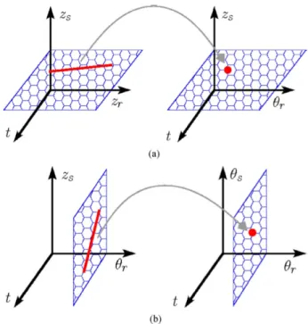
3.2 The schematic presentation of the double beamforming (a) The pressure fieldp(t,zr,zs)recorded on the received array is transformed intop(t,θr,zs) space (b) In second step, p(t,θr,zs) is transformed into p(t,θr,θs) space, whereθrdenotes the emitted angle. . . 30
3.3 The separation results of beamforming vs double beamforming (Crosses indicate the theoretical prediction values.) from [IRN∗09]: (a) two ray- paths are extracted from the FAF03data set [RKH∗04] at depthzs=87.3m andzr=39.3m; (b) the separation results of the two raypaths in (a) using beamforming; (c) the separation results of the two raypaths in (a) using double beamforming. . . 32
3.4 The expected source location is at 2 km in range and 34 m in depth. The Gibbs sampling approach produces a clear ambiguity surface with the main mode at the correct source location [Mic00].(a) Bartlett and (b) Gibbs sampling ambiguity surfaces for source location. . . 36
3.5 Array narrow model, sample matrix estimation, and data preconditioning for MFP . . . 40
15
3.6 Matched field processing (MFP) [KL04]. If you want to know where a singing whale locates at, first, the sound of the wave is recorded as an data vector; and then based on your sufficient accurate model of waveg- uide propagation, compare the recorded data from the singing wave, one frequency at a time, with the replica data. The location of highest cor- relation (the red peak in the fig. 3.6) denotes the estimated where the whale locates at. The feedback loop suggests a way to optimize the model.
Matched field processing can then be used in the context of ocean acoustic tomogtraphy [TDF91]. The data is from [KL04] [BBR∗96] . . . 43 3.7 the configuration of a TRM experiment . . . 44 3.8 (a) a signal is launched by a probe source and it excites a series of normal
modes that propagate to theTRM (b) a probe signal received by TRM.
[KKH∗03] . . . 47 3.9 (a) time reversal signals propagate backward to the probe source (b) a
focused signal observed by VRA. [KKH∗03] . . . 47 4.1 An example demonstrating the separation capability of beamforming and
MUSIC, where each peak represents a detected position of one signal.
(Red line denotes the MUSIC separation and the blue line of dashes shows the separation result of beamforming) . . . 55 4.2 (a) LV estimation result [MLBM05] (b) Q-MUSIC estimation result [MLBM06] 72 5.1 Subantenna structure of spatial smoothing . . . 86 5.2 Subband structure of frequential smoothing . . . 87 5.3 The point-array configuration explored to obtain the synthetic data . . . . 90 5.4 An experimental example of Recorded Signal (large time-window and
without noise) . . . 91 5.5 The separation result of an experimental example of Recorded Signal
(large time-window and without noise). (a) Separation results with Smoothing- MUSICAL. (b) Separation results with Beamforming. . . 92 5.6 The separation result of an experimental example of Recorded Signal
( Large time-window and without noise) (Mesh).(a) Separation results (mesh) with Smoothing-MUSICAL. (b) Separation results (mesh)with Beam- forming. . . 93 5.7 Part of recorded signal which includes the first two arrival raypaths (
Large time-window and without noise) . . . 93 5.8 The separation result of part of recorded signal (Large time-window and
without noise) (a) Separation results with Smoothing-MUSICAL. (b) Sep- aration results with Beamforming. (c) Separation results (mesh) with Smoothing-MUSICAL. . . 94 5.9 An experimental example of Recorded Signal (Small time-window and
without noise) (a) Recorded Signal (without noise). (b) Separation results with Beamforming. (c) Separation results with Smoothing-MUSICAL. . . 96
5.10 An experimental example of Recorded Signal (SNR=0dB) (a) Recorded Signal (SNR=0dB). (b) Separation results with Beamforming (SNR=0dB).
(c) Separation results with Smoothing MUSICAL (SNR=0dB). . . 97
5.11 An experimental example of Recorded Signal (SNR=-15dB) (a) Recorded Signal (SNR=-15dB). (b) Separation results with Beamforming (SNR=- 15dB). (c) Separation results with Smoothing MUSICAL (SNR=-15dB). . 98
5.12 An experimental example of Recorded Signal for real data obtained at small scale (a) Recorded Signal for real data obtained at small scale. (b) Separation results with Beamforming for real data obtained at small scale. (c) Separation results with Smoothing MUSICAL for real data obtained at small scale. . . 100
6.1 An experimental example of which the real number of raypaths equals 7 (a) Separation results using smoothing-MUSICAL withP=3. (b) Separa- tion results using smoothing-MUSICAL withP=5. (c) Separation results using smoothing-MUSICAL withP=7. . . 108
6.2 Profile of ordered noise eigenvalues for eight realizations (a) Profile of ordered noise eigenvalues estimated by 15 samples. (b) Profile of ordered noise eigenvalues estimated by 1025 samples. . . 116
6.3 Profiles of eigenvalue with two eigenvalues corresponding to raypaths. When the eigenvalue corresponding to raypath appears, a break exists between the profile of EFT and the profile of recorded eigenvalues. . . . 117
6.4 Profile of ordered eigenvalues in the first group of experiments when SNR =20dB (a) the received signals on15sensors. (b) Profile of ordered eigen- values estimated by 1025 samples. (c) Profile of ordered eigenvalues esti- mated by 15 samples. . . 118
6.5 Profile of ordered eigenvalues in the first group of experiments when SNR =5dB (a) the received signals on15sensors. (b) Profile of ordered eigen- values estimated by 1025 samples. (c) Profile of ordered eigenvalues esti- mated by 15 samples. . . 119
6.6 Profile of ordered eigenvalues in the second group of experiments when SNR = 20dB (a) the received signals on 15sensors. (b) Profile of ordered eigenvalues estimated by 1025 samples. (c) Profile of ordered eigenvalues estimated by 15 samples. . . 121
6.7 Experimental Setup of Small-scale Experiment in ISTerre . . . 124
6.8 (a) The received signals on 64 sensors for 5000 samples. (b) Separation result of beamforming with theoretical location for 64 samples. It pro- vides a reference value for checking the separation result of the proposed method. (c) Profile of ordered eigenvalues of64samples. . . 125
A.1 Deux principales ´etapes d’OAT . . . 139
A.2 Propagation Multiple Targets . . . 141
A.3 Structure d’antenne sous lissage spatial . . . 149
A.4 Structure de sous-bande pour le lissage fr´equentiel . . . 150 A.5 Configuration Point-Antenne permettant d’obtenir les donn´ees synth`etiques153 A.6 R´esultat de s´eparation sur un signal enregistr´e (grande fenˆetre de temps et
sans bruit). (a) Avec smoothing-MUSICAL. (b) Avec Formation de voie. (c) R´esultats de la s´eparation d’une partie du signal enregistr´e avec smoothing- MUSICAL. (d) R´esultats de la s´eparation d’une partie du signal enregistr´e avec Formation de voies. . . 154 A.7 Un exemple exp´erimental de signal enregistr´e (RSB =0dB) (a) les r´esultats
de s´eparation avec Formation de voie (RSB = 0 dB). (b)Les r´esultats de s´eparation avec smoothing-MUSICAL (RSB = 0 dB). (c) les r´esultats de s´eparation avec Formation de voie (RSB = -15 dB). (d)Les r’esultats de s´eparation avec smoothing-MUSICAL (RSB = -15dB). . . 155 A.8 Un exemple exp´erimental de signal enregistr´e pour les donn´ees r´eelles
obtenues `a petite ´echelle (a) Signal enregistr´e pour les donn´ees r´eelles obtenues `a petite ´echelle. (b) R´esultats de s´eparation avec formation de voies pour les donn´ees r´eelles obtenues `a petite ´echelle. (c) R´esultats de s´eparation avec smoothing-MUSICAL pour les donn´ees r´eelles obtenues
`a petite ´echelle. . . 157 A.9 Profil des valeurs propres ordonn´ees de bruit sur huit r´ealisations (a) Pro-
fil des valeurs propres ordonn´ees de bruit estim´es par 15 ´echantillons. (b) Profil des valeurs propres ordonn´ees de bruit estim´ee par 1025 ´echantillons.166 A.10Profils des valeurs propres avec deux valeurs propres correspondant aux
rayons. Lorsque la valeur propre correspond au rayons apparaˆıt, une rup- ture existe entre le profil de l’EFT et le profil des valeurs propres enreg- istr´ees. . . 166 A.11(a) R´esultat de la formation de voies avec emplacement th´eorique de 64
´echantillons. Il fournit une valeur de r´ef´erence pour v´erifier le r´esultat de s´eparation de la m´ethode propos´ee. (b) Profil des valeurs propres or- donn´ees de64 ´echantillons. . . 168
3.1 Comparison on the existing array-processing methods in underwater acous- tics based on different criteria ( Plane-wave and Experiment configuration )-I . . . 50 3.2 Comparison on the existing array-processing methods in underwater acous-
tics based on different criteria ( Statistical order and Computations)-II . . 50 4.1 Comparison of the existing high-resolution methods based on different
criterions (Consistency, Coherent Signals and Statistical Order)-I . . . 74 4.2 Comparison of the existing high-resolution methods based on different
criterions (Computation, Dimensional and Sensor Type)-II . . . 74 4.3 Comparison of the existing high-resolution methods based on different
criterions (Statistical Performance and Polarization Sensitivity)-IIII . . . . 74 4.4 Comparison of the existing high-resolution methods based on different
criterions (Prior knowledge of model order, Assumption of Signal Type and Array Geometries)-III . . . 75 6.1 Number of raypaths detected by AIC, MDL and EFT in the first group of
experiments (the real number of raypathsP=5) . . . 120 6.2 Number of raypaths detected by AIC, MDL and EFT in the second group
of experiments (the real number of raypathsP=5) . . . 120 A.1 Comparaison des diff´erentes m´ethodes de traitement d’antenne bas´ee sur
plusieurs crit´es ( Onde place and configuration de l’exp´erimentation )-I . 142 A.2 Comparaison des diff´erentes m´ethodes de traitement d’antenne bas´ee sur
plusieurs crit´es ( Statistique et temsp de calcul)-II . . . 143 A.3 Comparaison des m´ethodes `a haute r´esolution `a partir de different crit´eres
(Consistance, Coh´erence, Statistique)-I . . . 144 A.4 Comparaison des m´ethodes `a haute r´esolution `a partir de different crit´eres
(Calcul, imension, Type de capteurs)-II . . . 144 A.5 Comparaison des m´ethodes `a haute r´esolution `a partir de different crit´eres
(Performance statistique, Polarisation)-III . . . 145 19
A.6 Comparaison des m´ethodes `a haute r´esolution `a partir de different crit´eres (Connaissance de l’ordre, Hypoth´eses signal, G´eom´etrie de l’antenne)-IIII 145 A.7 Nombre de raypaths d´etect´es par l’AIC, MDL et l’EFT dans le premier
groupe d’exp´eriences (le nombre r´eel de trajets P=5) . . . 167 A.8 Nombre de raypaths d´etect´es par l’AIC, MDL et l’EFT dans le deuxi`eme
groupe d’exp´eriences (le nombre r´eel de raypaths P=5) . . . 167
Chapter 1
Introduction
Contents
1.1 Objectives . . . . 4 1.2 Outline . . . . 5
1
Ocean acoustic tomography is a technique which uses the time variation of sound propagation in the ocean to estimate the property variation of ocean, such as tempera- ture, salinity ... etc. This technique is first explored as a remote sensing method for large-scale ocean. After the cold war, the shallow water studies become very attractive.
In fact, the ocean acoustic tomography in a shallow-water wave guide at small scale has the same technique process as the one in deep water. That means it is also composed of the forward problem and the inverse problem. What is called the forward problem?
The sound propagates in the ocean through multiple paths. This property can provide more informations by that each raypath covers the different part of the ocean. However, when two raypaths arrive closely, the parameters, like travel time and direction of ar- rival, which contain these informations, can not be extracted directly and easily from the received signals. Because of this, some signal processing techniques are explored to separate the close raypaths and also to extract more raypaths. This is a process solving the forward problem. At the same time, the performance of inverse problem is based on the efficient solution of the forward problem. Thus, improving the performance of forward problem has great significance to finally obtain an efficient inversion results for ocean acoustic tomography.
Specifically, the analysis is begun from the recorded signal in a specific experiment configuration. At beginning and in the first experiment conducted by Munk, the signal is emitted by a point source and recorded by a single sensor (point to point configu- ration). The raypaths are separated by arrival time of each raypath. When these two raypaths arrive very closely, methods in this point to point configuration generally fail in correctly separating the raypaths. Consequently, beamforming has been applied to a configuration which is composed of one point source and a vertical array (point to array configuration) [MWW95] to obtain more information on raypaths. It can separate more close raypaths due to the added discrimination parameter—-the direction of ar- rival corresponding to each raypath on the vertical array. In order to further improve the performance of beamforming, more recently, a double-beamforming method was presented to solve the forward problem in an array to array configuration, which is com- posed of one source array and a received array. Inheriting the sprit of beamforming in the point to array configuration, this novel configuration can provide a new parameter—
the emitted angle as a discrimination variation. This method was first performed in a shallow-water wave guide [RCKH08] and then is applied to a shallow-water tomogra- phy problem [IRNM08] for getting correct simulation results. Finally, this shallow-water tomography based on double-beamforming was demonstrated by the experiment at an ultrasonic scale [RIN∗11]. Although double-beamforming has largely improved the res-
olution compared the beamforming, it still has the main drawback of beamforming: the low resolution ability.
Besides, there exist numerous approaches in underwater acoustic to source localiza- tion or geoacoustic inversion which also depend on the acurate raypaths extraction.
Thus, it is still quite necessary to present high resolution method for extracting more raypaths. Although our work in this dissertation is mainly focused on the forward problem of shallow-water acoustic tomography, it is possible to extend these methods similarly to solve the raypaths extraction problem to source localization or geoacoustic inversion or some other similar applications in underwater acoustics.
1.1 Objectives
Based on the discussion above, we want to achieve three major objectives in this disser- tation. Because these common forward problems of source localization, geoacoustic and ocean acoustic tomograghy, we will first give a comprehensive survey on corresponding signal processing methods which are already applied to these applications in underwa- ter acoustics, especially in shallow water. Advantages and limitations of each technique will be analyzed and compared. Then, a group of high resolution methods, which has been presented to overcome the resolution limitation of spectral-based algorithms, will be reviewed comprehensively. Through the study results of reviewing literatures, we further make the problems which we will solve in the context of shallow-water acoustic tomography specific and obvious. Finally, we propose a subspace-based high resolution method for separating the coherent raypaths in a shallow-water waveguide. (Two co- herent signals (or raypaths in our context) means: if one signal is a scaled and delayed version of the other. ) The corresponding state of art on coherent sources separation will be also reviewed. Subsequently, we pay attention to one of technique limitations of subspace-based methods. That is, they are all under the assumption of prior knowledge of model order. In our application context, it is the number of raypaths. Model order se- lection is an important problem in applications of model-based methods. There are few methods which are not based on the accurate estimation of covariance matrix and the assumption of spatially white noise. However, these two assumption are not easy to be satisfied in a practical perspective. Accordingly, we propose an exponential fitting test using short-length samples to automatically detect the number of raypaths. In addition, a noise whitening processing step is added to try to solve this problem in a practical shallow-water environment. This detection problem and our initial effort to try to find a solution will be analyzed and presented in Chapter6.
1.2 Outline
The remainder of this manuscript is organized as follows.
Chapter 2 first introduces some background knowledges on ocean acoustic tomog- raphy (OAT). These knowledges are the theoretical basis of our simulation experiment and real experiment at small scale. Then, the shallow-water environment is defined and we present the major characteristics of a general ocean acoustic tomography process in a shallow-water wave-guide. Moreover, the state of art on recent studies of shallow-water OAT is provided.
Because of the essential relationship between the existing signal processing methods in under water acoustics and the forward problem of shallow-water OAT, a survey on these methods is provided in Chapter3.
From the conclusions of reviewing literatures on both shallow-water studies and signal processing techniques, the resolution of signal processing method attract our at- tentions. Consequently, a comprehensive review of high resolution method is described in Chapter4. It is supposed that we can find or extend some high resolution methods to adapt to giving satisfied solutions in the context of shallow-water wave guide.
Chapter5presents a high resolution processing called smoothing-MUSICAL for co- herent raypaths, which is a combination of spatial-frequency smoothing and MUSICAL algorithm.
In Chapter6, we propose a noise-whitening exponential fitting test to correctly detect the number of raypaths in a shallow-water waveguide.
Chapter7 summarizes the contribution of the proposed algorithms and draws con- clusions of this manuscript. Some further works on the proposed algorithms are stated.
In addition, several future study directions concerning on signal processing techniques in underwater acoustics are described.
Chapter 2
Background knowledge on Ocean Acoustic Tomography
Contents
2.1 Fundamentals of Ocean Acoustics . . . . 10 2.2 Characteristic Sound Paths . . . . 12 2.3 Sound Propagation Models . . . . 14 2.3.1 Ray Theory . . . . 15 2.3.2 Parabolic Equation (PE) Model . . . . 16 2.4 General Technique Steps of OAT . . . . 18 2.5 OAT in Shallow Water Waveguide . . . . 19 2.5.1 Shallow Water . . . . 19 2.5.2 Recent Studies on Shallow water . . . . 20 2.5.3 Multiple RayPaths Propagation . . . . 22
7
A body of saline water is defined as an ocean or a sea. Approximately 71% of the planet’s surface ( 3.6×10⁸km2) is covered by several principal oceans and smaller seas.
Humans begin to acquire knowledge of the waves and currents of the seas and oceans in pre-historic times. Early modern exploration of the oceans was primarily for cartog- raphy and mainly limited to its surfaces and of the creatures that fishermen brought up in nets, though depth soundings by lead line were taken. With the development of fur- ther study of oceans, oceanography also called oceanology or marine science is formed, which covers a wide range of topics referring to multiple disciplines, such as biology, chemistry, geology, meteorology, and physics as well as geography. As a key branch of oceanography, physical oceanography study the physical conditions and physical pro- cesses within the ocean, especially the motions and physical properties of ocean waters.
The motivation of studying the physics of the ocean depends on three major factors.
The first one is that oceans are the main supply source for the fishing industry. For exam- ple, some of the more important ones are shrimp, fish, crabs and lobster. In addition, the oceanic weather, such as temperature changes and currents, fertilizes the sea. Hence we are interested in the processes which influence the sea just as farmers are interested in the weather and climate. Secondly, the oceans are essential and crucial to transportation:
most of the world’s goods move by ship between the world’s seaports. These activities are influenced by the physics process of the oceans, especially waves, winds, currents, and temperature. The last and important one is that the study of the oceans is linked to understanding global climate changes, potential global warming and related biosphere concerns. Specifically, the interaction of ocean circulation, which serves as a type of heat pump, and biological effects such as the concentration of carbon dioxide can result in global climate changes on a time scale of decades. Known climate oscillations resulting from these interactions include the Pacific decadal oscillation, North Atlantic oscillation, and Arctic oscillation. The oceanic process of thermohaline circulation is a significant component of heat redistribution across the globe, and changes in this circulation can have major impacts upon the climate.
For analysis and studies of physical properties of the ocean, oceanography has es- sentially two types of techniques. On the one hand, direct measurement of physical properties such as conductivity, temperature or density of the sedimentary layers are available. These instruments allow to have relevant information on backgrounds, but they present significant cuts to use and provide a very limited spatial sampling with respect to size of physical phenomena to be studied.
On the other hand, less investigative techniques exist. They consist in a wave prop- agating in the ocean environment, for approximating physical properties from the in-
teraction between the medium and the wave that is propagated. These techniques can have a better sampling space, but their reliability is often more unreliable than direct measurements.
Practically, there are two types of waves which have been utilized in the indirect measurements of the physical properties of ocean. Concretely, in order to study the ocean surface (the sea state, surface waves, ...), many methods using electromagnetic waves have been developed. Unfortunately, these waves can not be exploited to analyze the internal structures (outside surface) due to their high attenuation in the water. In this case, sound waves, much less attenuated, are the only medium that allows us to image the submerged part of the oceans.
As discussed above, the oceans are opaque to most electromagnetic radiation, but there is a strong acoustic waveguide and sound can propagate for 10 Mm with distinct multiply-refracted raypaths. Consequently, ocean acoustic tomography (OAT) was pro- posed in1979by Walter Munk and Carl Wunsch [MW79][MWW95] as one of important indirect techniques on studying physical properties of oceans. It is an analogue to X-ray computed axial tomography for the oceans. A quick briefing of this technique process is given as: the acoustic signal is first emitted by a point source; then, transmitting broad- band pulses (particularly sound at low frequencies, i.e., less than a few hundred hertz.) in the ocean leads to a set of impulsive arrivals at the receiver which characterize the impulse response of the sound channel. The peaks observed at the receiver are assumed to represent the arrival of energy traveling along geometric ray paths. These raypaths can be distinguished by several parameters, such as arrival time and arrival angle, etc, depending on the experiment configuration. Variations in these parameters can be used to infer changes in ocean structure. This will be explained in detail in Section 2.4.
In this chapter, we first introduce the fundamental knowledge of ocean acoustics. In Section 2.2, the characteristic of sound propagation is studied in both deep water and shallow-water. Section 2.3 presents two basic sound propagation models. Section 2.4 illustrates the general technic steps of OAT. Finally, we introduce recent research works in shallow water and the specific problem is encountered by OAT in shallow water in Section2.5.
2.1 Fundamentals of Ocean Acoustics
It has been pointed out that the ocean can be considered as an acoustic waveguide. It is a waveguide limited above by the sea surface and below by the seafloor. The speed of sound in the waveguide plays the same role as the index of refraction does in optics.
The sound speed in the ocean increases with the increasing of pressure, temperature and salinity. As the pressure is a function of depth, the dependence of sound speed and three independent variables [Bae81] is expressed as Equation A.1:
c=1449.2+4.6T−0.055T2+0.00029T3+ (1.34−0.01T)(S−35) +0.016z (2.1) where
• cis sound speed.
• T represents temperature in degrees centigrade.
• Sexpresses the salinity in parts per thousand.
• zis depth in meters.
The sensitivity of sound speed to salinity is generally much smaller than that of either temperature or pressure. In non-polar regions, the oceanographic properties of the water near the surface result essentially from mixing due to wind and wave activity at the air-sea interface and this near-surface mixed layer has a constant temperature.
Hence, in this isothermal mixed layer we have a sound-speed profile which increases with depth because of the pressure gradient effect. This is the surface duct region, and its existence depends on the near-surface oceanographic conditions. Note that the more agitated the upper layer is, the deeper the mixed layer and the less likely will there be any departure from the mixed-layer part of the profile depicted in Figure. 2.1. Thus, an atmospheric storm passing over a region mixes the near-surface waters so that a surface duct is created or an existing one deepened or enhanced.
The midlatitude ocean is warmest near the surface and the temperature drops off rapidly in the upper 200 to 700 m, forming the ocean main thermocline and greatly decreasing the sound speed. Below the main thermocline, the ocean temperature de- creases very slowly with depth and the increasing pressure with depth dominates the sound speed, creating a minimum in sound speed at the bottom of the main thermo- cline. However, in polar regions, the water is coldest near the surface and hence the minimum sound-speed is at the ocean-air interface as indicated in Figure. 2.1. In shal- low water (continental shelf regions) with water depth in the order of a few hundred meters, only the upper part of the sound-speed profile in Figure. 2.1 is relevant. This upper region is dependent on season and time of day, which, in turn, affects sound propagation in the water column. Specifically, in a warmer season (or warmer part
of the day), the temperature increases near the surface and hence the sound speed in- creases toward the sea surface. This near surface heating (and subsequent cooling) has a profound effect on surface-ship application. For instance, for surface-ship sonars, the di- urnal heating causes poorer sonar performance in the afternoon–a phenomenon known as the afternoon effect. The seasonal variability, however, is much greater and therefore more important factor with respect to underwater acoustic.
Figure2.1: Generic Sound Speed Profiles [SRD∗07]
2.2 Characteristic Sound Paths
The schematic of the basic types of propagation in the ocean is shown by Figure. 2.2, which results from the sound-speed profiles (indicated by the dashed lines) discussed in Figure. 2.1. Mathematically, these sound paths can be understood from Snell’s law,
cosθz
cl =const (2.2)
where θz indicates the propagation angle of ray at depth z with respect to the hor- izontal and cl is the local sound speed. This law implicates that sound bends locally toward region of low sound speed.
Figure 2.2: schematic representation of basic types of sound propagation in the ocean [SRD∗07]
The simplest cases to explain are the paths about local sound speed minima: path1, path2, and path3. Among these three types of paths, paths1and2correspond to sur- face duct propagation where the minimum sound speed is beneath the ice cover for the Arctic case or at the ocean surface. The ray leaving a deeper source at a shallow horizon- tal angle depicts path 3, which propagates in the deep sound channel whose axis is at the shown sound speed minimum. As shown in Figure2.2, this local minimum converg- ing to the Arctic surface minimum (path1) tends to become more shallow toward polar latitudes. Moreover, because sound in the deep channel for mid-latitudes has few inter- actions with lossy boundaries, it can propagate over long distances. In particular, many ocean exploration technique in deep water, such as ocean acoustic tomography of large scales, are based on this property of low-frequency propagation via this path, which has been observed to distances of thousands of kilometers. Also, it can be expected that the shallow sources combined with the water column at polar latitudes will tend to propagate more horizontally around an axis based on both the geographical variation of the acoustic environment and Snell’s law. There exists a type of convergence zone propagation —- path4with slightly steeper angles than those of path3. These conver- gence zones of high intensity near the surface, which is caused by the upward refracting nature of the deep sound-speed profile, is produced by a spatially periodic (35-70km) refocusing phenomenon.
Another periodic phenomenon exists as path5. It is reflected by the ocean bottom, so the sound path with energy losses propagates in a shorter cycle distance and a shorter
total propagation distance. Finally, in a shallow-water region such as a continental shelf, the sound (depicted in the right-hand-side of Figure2.2) is channeled in a waveguide reflected by the ocean both surface and bottom. Because of the reflection of the bottom, negative critical depth environments exhibit much of the sound propagation physics descriptive of shallow-water environments. It is also the path propagation based on which the work of my thesis is discussed.
There exists an alternative classification of raypaths in the ocean, which classifies raypaths into four types:
1. Refracted Refracted (RR) rays (path3):rays propagating via refracted path only.
2. Refracted Surface Reflected (RSR) rays (paths 1,2, and4): refracted rays bouncing off the sea surface.
3. Refracted Bottom-Reflected (RBR) rays (path5) : rays bouncing off the seafloor.
4. Surface-Reflected Bottom-Reflected (SRBR) rays: (path6)rays reflected off both the sea surface and the seafloor.
The RR paths have no boundary losses because they are only affected by attenuation and scattering within the water column. At the same time, it is obvious that the SRBR paths are the most lossy since they are subjected to all of the loss mechanisms present in the ocean waveguide.
2.3 Sound Propagation Models
The wave equation is derived to describe sound propagation. Concretely, it is obtained from the equations of hydrodynamics and its coefficients and boundary conditions. The computer solutions to the wave equation [JKP∗95] are called sound propagation models.
They are developed so as to perform and describe sound propagation in the sea by computer simulation. Normally, there are four types of sound propagation models:
ray theory, the spectral method or fast field program (FFP), normal mode (NM) and parabolic equation (PE). These models consider not only the ocean variation with depth but also those in horizontal direction (range-dependent). The appropriate choice of sound propagation models differs from the value of frequencies. If the frequencies are a few kilohertz or above, ray theory is mainly used. While the other three model types are more applicable and useable in the cases that the frequencies are below1kHz. If the frequency is between these frequencies, we can choose either of them.
A solution of wave equation with the cylindrical coordinates in frequency domain for a frequency binνis called the Helmholtz equation (K≡2πν/c). It is given by:
52pC(rC,z) +K2HpC(rC,z) =0 (2.3) where the pressure pC in cylindrical coordinates with the range coordinates denoted byrC = (x,y)and the depth coordinate denoted by z (taken positive downward) for a source-free region.
with
K2H(rC,z) = (2πν)2
c2(rC,z). (2.4)
describing the variation of propagation environment in horizontal direction.
For an acoustic field obtained from a point source, the Helmholtz equation is de- scribed as:
52G(rC,z) +K2H(rC,z)G(rC,z) =−δ2(rC−rs)δ(z−zs) (2.5) where the subscript Cs denotes the source coordinates. As we mentioned at the begin- ning of this section, there are four types of propagation models. Actually, here, they are divided into four types depending on the method of acquiring the solution of Green’s function G. Spectral method or normal modes is obtained by solving the boundary- value problem of Equation 2.5 while ray theory model and parabolic equation model are obtained by using an initial value to approximate Equation 2.5. As two represen- tatives, we will briefly introduce ray theory and Parabolic Equation (PE) Model, which will be used in following chapters to generate the synthetic data sets of our experiments.
2.3.1 Ray Theory
Ray theory approximate the Equation2.5 geometrically in high-frequency. It is mostly utilized in the deep-water environment and also applied to shallow water for some specific purposes. Mathematically, it is described by:
G(rC,z) =Ae(rC,z)e[iPh(rC,z)] (2.6) where Ae(rC,z) is the amplitude envelope, and Ph is the phase (eikonal). Curves or- thogonal to the iso-phase surfaces are called rays. Both the amplitude and eikonal are functions of the spatial coordinates (rC,z). Moreover, A(rC,z) varies with the spatial coordinates (rC,z) slowly compared with the exponential term including the phase S.
Since the amplitude varies slowly with the spatial coordinates (i.e.,(1/A)52A K2), the corresponding eikonal equation (geometrical approximation) yielded from 2.3 has the well-known form:
(5Ph(rC,z))2 =K2H (2.7) and the ray trajectory can be given mathematically by:
d
d(la)(KH dR
d(la)) =5KH (2.8)
where la is the length of the curve along the direction of the ray d(la) = q
dr2C+dz2 and vd = (rC,z) is the displacement vector to a point on the ray. The density of rays is utilized to compute the direction of average flux (energy) at any point according to that of the trajectories and the amplitude of the field. The ray theory is applicable to both depth-dependence and range dependence environments. The advantages of ray theory are the rapid computation velocity and making the acoustic propagation visible not only in shallow and deep water but also in mid-latiutde to polar regions. That is, the ray traces provide a physical view of the acoustic paths, which is useful to describe the acoustic propagation paths, especially over long distance. On the other hand, the classical ray theory has limitations as without considering the diffraction and the effects describing the low-frequency dependence.
2.3.2 Parabolic Equation (PE) Model
The Parabolic Equation (PE) method, which is based on the geometrical configurations that naturally arise in the sound channel mode of propagation, is unarguably one of the most useful approximations for solving the problem of wave propagation in inhomo- geneous media. PE in underwater acoustics is an extension of a method first invented by Leontovich and Fock (1946) [also see Fock (1965)] in the propagation of radio wave [LF46] [Foc65], in which waves propagation in certain preferred directions were studied.
The extension to acoustic waves was first done by Tappert (1977) [Tap77] and since has been extended by many other authors attempting to improving the applicability and accuracy. If the angle with respect to horizontal is small, for instance:
|θz| ≈ |z−zs|<<1 (2.9)
wherezsis the source depth. then we may use the approximation:
p(rC,z) =ψ(rC,z)√1
rCeiK0HrC (2.10) WhereK0H is the number of horizontal wavenumber.
and we define K2H(rC,z)≡ K20(n(rC,z))2,n(rC,z)therefore being an index of refrac- tionc0/c, where c0is a reference sound speed. Substituting equation2.10 into equation 2.3and invoking the paraxial (narrow-angle) approximation,
∂2ψ
∂rC2 2K0∂ψ
∂rC (2.11)
we obtain the parabolic equation (inrC),
∂ψ2
∂z2 +2iK0H ∂ψ
∂rC +K0H(n2−1)ψ=0 (2.12) As we known, the standard numerical method to solve the above equation is to utilize the split-step range-marching algorithm. It is first introduced in [Tap77]. Then, there are some modifications and extensions to higher-angle propagation [Col93a], elastic media [Col93b] and so on. In addition, the solution for ψ(rC,z)based on this split-step range- marching algorithm, actually which exploys the fast Fourier transform to calculate the second-order spatial derivatives of the pressure field, is shown as follows:
ψ(rC+∆rC,z) =exp[iK
0H
2 (n2−1)∆rC]Ftr−1× {[exp(−i∆rC
2K0HKzH2)]Ftr[ψ(rC,z)]} (2.13)
In Equation 2.13, the Fourier transforms Ftr are performed using FFTs. However, there are errors introduced by this split-step range-marching algorithm. For example, in this method, one marching step of the solution is completed by splitting it into two sub-steps sequentially, not simultaneously, and solving for free space propagation and phase anomaly. Because of the sequential splitting, errors can arise from the neglected cross terms. Recently, several attempts have been done on the proposals to reduce such errors and accomplished the extension to a three-dimensional Cartesian parabolic- equation model with a higher-order approximation to the square-root Helmholtz oper- ator [Dud06] [LD12] .
2.4 General Technique Steps of OAT
Over the past decade, it has been increasingly aware of that ” the ocean weather ” is su- perimposed on ”the ocean climate” by the oceanographers. Generally, the ocean weather is defined as an intense and compact ocean ’mesoscale’ eddy structure and sluggish large scale circulation is called ocean climate. Unfortunately, traditional ship-based ob- serving systems are not adequate for monitoring the ocean at mesoscale resolution (for example: a 300km × 300km) [BBB∗82]. Thus, to fully represent atmospheric weather, ocean acoustic tomography was introduced by Munk and Wunsch [MW79][MWW95] as a remote-sensing technique for large-scale monitoring of the ocean interior using low- frequecy sound.
In the original conception of the method, measuring the travel times of sound pulses is the first step. Classically, the sound is emitted by a source and recorded by a receiver or a vertical array composed by several receivers. We call these two configurations respectively point-point and point-array. The sound pulse corresponding to each ray needs to be separated. This is the process of extraction of observation from the recorded data. (shown in the left-hand-side of the Fig. A.1). In the point to point configura- tion, the sound pulses are usually separated by time of arrival while in the point to array configuration, the reception angle are also provided as a discrimination parame- ter. Simultaneously, the pulse arrival corresponding to each ray can be calculated from the known physical parameters of a fixed physical propagation model (shown in the right-hand-side of the Fig.A.1) or from ray-tracing programs.
Then, the identification is performed by matching these two types of rays arrivals.
In the ray approximation, the observed arrival time change can be ascribed to sound speed changes along the ray path corresponding to the arrival. Although the intensity of the arrival peaks can vary strongly due to the influence of internal wave variability, the arrival times are stable and many can be tracked over a year-long experiment. Sound speed is related to ocean temperature (and weakly to salinity), so the ocean temperature field can be estimated from arrival time measurements over multiple paths. This is some analogy with computerized tomography (CT): multiple sectional X-rays from a source and receiver which are rotated around the patient, and are processed by computer to yield two dimensional displays of the interior structure.
Figure2.3: Two Main Steps of OAT
2.5 OAT in Shallow Water Waveguide
2.5.1 Shallow Water
The definition of shallow water is that the region from the end of the surf zone out to the continental shelf break. Practically, the typical shallow-water environments are found on the continental shelf for water depths down to 200m. The important moti- vation of research on shallow water acoustics is that it has great contributions to naval defense issues (for instance, Anti-submarine warfare (ASW) and mine warfare (MWF)).
However, at the present, shallow water acoustic techniques are widely used in biology (marine mammals and fish), geology (seabed properties and mapping), and physical oceanography (temperature and current measurements). Besides, the underwater sound in shallow water are also used in commercial and industrial applications (shipping and oil exploration).
Indeed, shallow water is a different environment from deep water. Firstly, it is a far more complicated acoustic medium than deep water, because in shallow water, all the important factors, such as the surface, column, and bottom properties, are spatially varying. At the same time, the oceanographic parameters are also temporally varying.
Furthermore, the principal characteristic of shallow water propagation is that the sound wave is refracted or reflected by the surface and or the bottom. These interactions change the physical properties of sound and in particular cause the lossy of energy. For example, in the summer, there is a warm surface layer causing downward refraction
and hence repeated bottom interaction for all ray paths. Since the seafloor is a lossy boundary, propagation in shallow water is dominated by bottom reflection loss at low and intermediate frequencies(<1kHz)and scattering losses at high frequencies.
Another different aspect of shallow water acoustic is caused by the physical phe- nomena existing in the coastal ocean. Coastal fronts, eddies, internal waves (linear and nonlinear), create structure on a variety of scales to affect significantly acoustics in the frequency range we are interested in.
Fish and marine mammals, most of which live in shallow water environment, not only make more noise but also could absorb and scatter sound. It also makes shallow water be a different medium from deep water for acoustic propagation.
The last main difference that should be noted is the stronger 3D effects in shallow water (both random and deterministic ones). In shallow water, the slope of the shelf, the shelf break and the canyons can have significant 3D acoustic effects. Moreover, horizontal refraction by the water column itself can also be appreciable, as has been seen recently by both theory and experiment. In deep water, only the bathymetry of seamounts and islands is a serious3D acoustic concern, a very limited bit of the ocean’s area.
2.5.2 Recent Studies on Shallow water
Based on the practical importance and theoretical difference discussed above, oceanog- raphers shifted the study focus again to shallow water after the cold war. The efforts of researchers are paid to both theoretical and experiments study.
Theoretically, the four popular theories introduced in Section 2.3 (normal modes, rays, parabolic equation, wavenumber integration) have been improved and refined in the context of shallow water [Pie65][Mil69][TW80][MW83]. For example, as an extension of Normal mode theory, coupled normal mode theory [Pie65][Mil69] is introduced to deal with the range dependence of the medium in a slice between source and receiver, and even fully3D effects in theory.
On the other hand, experimental efforts in shallow water have been made by re- searchers on several aspects. Let us begin with the oceanography. Several experi- ments (the 1992Barents Sea Polar Front experiment [LJP∗96], the1996-1997Shelf break PRIMER experiments, and the recent (2006) SW06 experiment [TML∗07]) on the study of coastal fronts are performed, because the drastic change in the acoustic field strength going across a front.
The researchers have also examined the strong mode coupling by internal waves, par-
ticularly nonlinear coastal internal waves in numerous recent experiments. A sampling of those experiments includes the 1995 Shallow Water Acoustic Random Medium ex- periment (SWARM) [ABC∗97], the1995-1996PRIMER experiments [GPL∗97] [GBB∗04], the 2000-2001 Asian Seas Acoustics Experiment (ASIAEX) [DZM∗04], and the recent Shallow Water2006(SW06) experiment [TML∗07].
Thirdly, experiments as the 1985GEMINI cruises off Corpus Christi, Texas, [CKS92] and the above-cited PRIMER [GPL∗97] [GBB∗04] and ASIAEX [DZM∗04] demonstrated new methods to obtain bottom properties based on acoustic data.
To avoid the technical limitations of large scale experiments, a series of small scale experiments using broadband acoustic signal [RCKH08] [RKH∗04] [RJF∗01] [KEK∗01] [KKH∗03] [EAH∗02] [KHS∗98] [HSK∗99] has been performed. The typical range of these experiments are from1to8km in a50-120m deep waveguide.
Besides, as an recent active area of signal processing technology, time-reversed acous- tics [Fin97] [Fin99] [FCD∗00] are studied a lot.The time reversal technique is based upon a feature of the wave equation known as reciprocity: given a solution to the wave equa- tion, then the time reversal (using a negative time) of that solution is also a solution.
This occurs because the standard wave equation only contains even order derivatives.
The media are not (e.g. very lossy or noisy media), acoustic waves in water or air are approximately reciprocal and linear. Another way to think of a time reversal experiment is that the time reversal mirror (TRM) is a ”channel sampler”. The TRM measures the channel during the recording phase, and uses that information in the transmission phase to optimally focus the wave back to the source. This property is first used in underwater communications of shallow water [EAH∗02].The experimental results obtained between two source/ receive arrays [EAH∗02].
Inspired by the two dimensional configuration, time-delay beamforming is performed simultaneously on both the source and receive arrays to separate the ray paths in the context of shallow water tomography [RCKH08]. Then, the shallow water acoustic tomography performed from double-beamforming algorithm is demonstrated by both simulation results [IRNM08] [IRN∗09] and experiment results [RIN∗11].
In [IRNM08], they extract efficiently source and receive angles as well as travel times of ray paths by applying the double-beamforming algorithm on two arrays. From these information of ray paths, a uniform coverage of the waveguide by the ray paths is ob- tained, from which sound-speed fluctuations are reconstructed using a ray-based direct tomography model.
In [RIN∗11], a feasibile OAT in a shallow ultrasonic waveguide is demonstrated at the laboratory scale between two source-receiver arrays. At a 1/1000 scale, the waveg-
uide represents a 1.1 km long, 52-m deep ocean acoustic channel in the kilohertz fre- quency range. Two coplanar arrays record the transfer matrix in the time domain of the waveguide between each pair of source-receiver transducers. A time-domain, double- beamforming algorithm is simultaneously performed on the source and receiver ar- rays that projects the multi-reflected acoustic echoes into an equivalent set of eigenrays, which are characterized by their travel times and their launch and arrival angles. Travel- time differences are measured for each eigenray every 0.1 s when a thermal plume is generated at a given location in the waveguide.
Using DBF is a clear advantage because the tomography inversion benefits from the identification of a large number of acoustic eigenrays, which cover the whole acoustic waveguide. Travel-time tomography inversion is then performed using two forward models based either on ray theory or on the diffraction-based sensitivity kernel. The travel-time sensitivity kernel (TSK) applied to travel-time fluctuations after DBF takes advantage of the limited bandwidth of the acoustic signals. Compared to tomography data based on ray theory that are no longer relevant at low frequencies, this provides diffraction-limited spatial accuracy in range and depth. The spatially resolved range and depth inversion data confirm the feasibility of acoustic tomography in shallow water.
2.5.3 Multiple RayPaths Propagation
Figure2.4: Multiple Ray Paths Propagation
In Fig. A.2, an example on raypaths propagation is shown in the configuration of one source and one vertical array. As discussed in Section 2.5.2, in shallow water a beam of rays launched by a source will be refracted or reflected above by the surface and / or down by the continental shelf or refracted in the water. Thus, each ray will follow a different path and provide the information to the OAT. More ray paths can
provide more information by covering the different range of the propagation medium.
However, multiple propagation also produces interferences between them. That is why we need the signal processing technology in the OAT, at the same time, the separation and further identification of ray paths becomes an important step of OAT( shown in Fig.
A.1). depending on the complexity of the sound-speed structure, distinct wave front arrivals may seem to share the same arrival angle and time on the receive array due to the resolution limits imposed by the pulse bandwidth and the array size.
Chapter 3
Array Processing in Underwater Acoustics
Contents
3.1 Sampling and Digitization Techniques . . . . 27 3.1.1 Plane-Wave Beamforming . . . . 27 3.1.2 Adaptive Beamformers (Maximum-likelihood method (MLM)) . 28 3.1.3 Double Beamforming . . . . 29 3.1.4 A Gibbs sampling localization-deconvolution approach . . . . . 31 3.1.4.1 Signal model in time domain . . . . 33 3.1.4.2 Gibbs sampler . . . . 33 3.2 Directly from the received signals . . . . 37 3.2.1 Matched Field Processing . . . . 37 3.2.1.1 Green’s functions . . . . 37 3.2.1.2 Signal Models . . . . 38 3.2.1.3 Noise Models . . . . 38 3.2.1.4 Sample covariance estimation . . . . 39 3.2.1.5 The Conventional (Barlett) Beamformer . . . . 41 3.2.1.6 Maximum-likelihood method MFP . . . . 41 3.2.2 The Time Reversal Mirror . . . . 42 3.2.3 Discussion on matched-field processing and phase conjugation
of time reversal mirror . . . . 48 3.3 Discussion and comparison . . . . 49
25
From the investigation of the Chapter 2, we can conclude that the shallow-water OAT is a vey active research topic in recent studies on oceans. In addition, the separa- tion resolution of the forward problem of OAT is still needed to be improved. This also belongs to source localization or separation problems usi
![Figure 2 . 1 : Generic Sound Speed Profiles [SRD ∗ 07 ]](https://thumb-eu.123doks.com/thumbv2/1bibliocom/472968.75947/33.892.194.657.335.863/figure-2-generic-sound-speed-profiles-srd-07.webp)
![Figure 2 . 2 : schematic representation of basic types of sound propagation in the ocean [SRD ∗ 07 ]](https://thumb-eu.123doks.com/thumbv2/1bibliocom/472968.75947/34.892.194.742.254.484/figure-schematic-representation-basic-types-sound-propagation-ocean.webp)

![Figure 3 . 3 : The separation results of beamforming vs double beamforming (Crosses in- in-dicate the theoretical prediction values.) from [IRN ∗ 09 ]: (a) two raypaths are extracted from the FAF 03 data set [RKH ∗ 04 ] at depth z s = 87.3m and z r = 39.3m](https://thumb-eu.123doks.com/thumbv2/1bibliocom/472968.75947/53.892.124.800.236.925/separation-beamforming-beamforming-crosses-theoretical-prediction-raypaths-extracted.webp)
![Figure 3 . 4 : The expected source location is at 2 km in range and 34 m in depth. The Gibbs sampling approach produces a clear ambiguity surface with the main mode at the correct source location [Mic 00 ].(a) Bartlett and (b) Gibbs sampling ambiguity surf](https://thumb-eu.123doks.com/thumbv2/1bibliocom/472968.75947/57.892.145.702.293.913/expected-location-sampling-approach-produces-ambiguity-bartlett-ambiguity.webp)
![Figure 3 . 6 : Matched field processing (MFP) [KL 04 ]. If you want to know where a singing whale locates at, first, the sound of the wave is recorded as an data vector;](https://thumb-eu.123doks.com/thumbv2/1bibliocom/472968.75947/64.892.165.815.345.774/figure-matched-field-processing-singing-locates-recorded-vector.webp)


