[PENDING] Simple Algorithm for Simple Timed Games Yasmina Abdeddaim, Eugene Asarin, Mihaela Sighireanu

(1)

HAL Id: hal-00374700

https://hal.archives-ouvertes.fr/hal-00374700v2

Preprint submitted on 13 Apr 2009

HAL

is a multi-disciplinary open access archive for the deposit and dissemination of sci- entific research documents, whether they are pub- lished or not. The documents may come from teaching and research institutions in France or abroad, or from public or private research centers.

L’archive ouverte pluridisciplinaire

HAL, est

destinée au dépôt et à la diffusion de documents scientifiques de niveau recherche, publiés ou non, émanant des établissements d’enseignement et de recherche français ou étrangers, des laboratoires publics ou privés.

Simple Algorithm for Simple Timed Games

Yasmina Abdeddaim, Eugene Asarin, Mihaela Sighireanu

To cite this version:

Yasmina Abdeddaim, Eugene Asarin, Mihaela Sighireanu. Simple Algorithm for Simple Timed Games.

2008. �hal-00374700v2�

(2)

Simple Algorithm for Simple Timed Games

^?

Y. Abdedda¨ım¹, E. Asarin², and M. Sighireanu²

1Department of Embedded Systems, ESIEE Paris, University of Paris-Est Cit´e Descartes, BP 99, 93162 Noisy-le-Grand Cedex, France

2 LIAFA, University Paris Diderot and CNRS, 75205 Paris 13, France.

y.abdeddaim@esiee.fr, {asarin,sighirea}@liafa.jussieu.fr

Abstract. We propose a subclass of timed game automata (TGA), called Task TGA, representing networks of communicating tasks where the system can choose when to start the task and the environment can choose the duration of the task. We search to solve finite-horizon reachability games on Task TGA by building strategies in the form of Simple Temporal Networks with Uncertainty (STNU). Such strategies have the advantage of being very succinct due to the partial order reduction of independent tasks. We show that the existence of such strategies is an NP-complete problem. A practical consequence of this result is a fully forward algorithm for building STNU strategies. Potential applications of this work are planning and scheduling under temporal uncertainty.

1 Introduction

Timed Game Automata (TGA) model has been introduced in [20] in order to represent open timed systems, and is nowadays extensively studied both from a theoretical and applied viewpoints. As usual in the game theory, main problems for timed games are (1) search for winning strategies that allow to the protagonist player (or the controller) to reach his or her aims whatever the opponent player (or the environment) does, and (2) search for winning states (from which such a strategy exists). A winning strategy can be interpreted as a control program that respects its specification (or maximizes some value function) for any actions of the environment, and for this reason game-solving for TGA is often referred to as controller synthesis. Such a synthesis finds applications to, e.g., industrial plants [23], robotics [1], or multi-media documents [16].

A large class of applications of timed games, relevant to this work, is scheduling and planning under temporal uncertainty (see [3, 11]). For this kind of applications, the protagonist masters all the behaviour of the system, except the durations of its actions. The aim is to ensure a good functioning of the system for any timing (decided by the opponent/environment player in some predefined bounds). Thus a strategy is a control program, schedule or plan robust to timing variations in the controlled process. During the last decade, the planning community has developed several techniques for timed planning problems.

?This work has been supported by the French ANR project AMAES.

(3)

These techniques (e.g., [17]) are based on constraint programming and give good performances in practice.

On the other hand, during first years of timed games, a major difficulty was related to the fast state explosion and non-scalability of algorithms and tools. Theoretically, this is not surprising since the upper bound complexity of solving reachability games on TGA has been proved EXPTIME [15]. But the main reason of these bad performances was that most algorithms explored (in a backward way [20, 2], or in a mixed one [23]) almost all the huge symbolic state space of the timed game automaton. Four years ago, an important practical progress in timed strategy synthesis has been attained by Cassez et al. [8], who adapted to the timed case a forward on-the-fly game-solving algorithm from [18], and implemented the resulting algorithm in the toolUppaal-Tiga[6]. This tool has a performance comparable to reachability analysis of timed automata, and thus makes timed game solving only as difficult as timed verification. However, in many practical cases, even this solution is not always satisfactory. One issue is still the state explosion preventing the tool from finding a strategy. Another issue is a big size and complexity of the strategy synthesized. It is often too heavy to be deployed on the controller. For distributed systems, the controller has to be centralized because the strategy obtained is difficult to distribute. Partial order based methods [7, 19] could help, but as far as we know, they have not yet been applied to timed games.

In this paper, we give a formal explanation of the good results obtained by the planning community by (1) identifying a game model for the timed planning problems and by (2) showing that the complexity of solving such games becomes NP-complete if we search to build strategies of a special form. As a consequence, we obtain a fully forward algorithm for solving timed games by building compact and easy to distribute strategies.

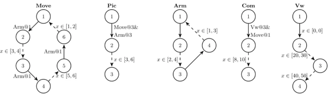
More precisely, we consider games played on a special kind of TGA, so-called task timed game automata(TTGA). Such an automaton is a parallel composition of several TGA called tasks. In every task, the controller executes a (possibly infinite) sequence of steps. At each step, the controller decides when to launch some actions whose durations are chosen by the environment and it waits the end of actions launched before starting the next step. Figure 1 gives an example of a TTGA with five tasks. The taskMoverepeats three steps infinitely, at each step the controller launches one action using the controllable transition (solid arrow); the duration of this action is chosen by the environment in the interval given on the uncontrollable transition (dashed arrow). Notice that, in our games, the environment (the opponent player) has no discrete choice, it determines only some durations. The controller has only the choice of the task to execute, but tasks cannot do discrete choices. The aim of the controller is to reach some set of goal states before some deadline (the horizon of the game), and never leave the set of safe states until this goal.

For such games, we will consider strategies of a certain form. First, we dis- allow “conditional moves”, i.e., the discrete choices of the controller are fixed, and the only way that it reacts to the choices of the environment is by adapting

(4)

the time at which it launches its actions. This requirement limits somewhat the power of the controller. For example, we are not able to obtain optimality like in [2] because this needs conditional schedulers. Second, instead of a memory- less strategy saying for each state what to do (like in almost all the papers/tools on timed games), we represent a strategy by a compact data structure, called STNU [24], and a computational procedure saying for every game history what are possible next moves for the protagonist. In [1] we show that such a strategy is, by its nature, a more complex object than the usual “state feedback”

(or memory-less), but it is in most cases smaller wrt the number of transitions needed to reach the goal, more permissive wrt the number of runs included, and easier to distribute in a multi-component timed system (although some parts of the execution shall be centralized).

Related work. A data structure similar to STNU, called event zones, has been used in [19] for the verification of timed automata. STNU extend event zones with uncontrollable edges. The IxTeT planner [13] uses the STNU data structure and an A^∗-like search algorithms to obtain STNU plans from constraint-based specification. Our work gives a TGA model sufficient and yet more expressive for modeling pure¹ timed planning problems considered by IxTeT. Moreover, the completeness of the algorithm used byIxTeT, even for pure timed planning problems, has been a conjecture. We provide here a proof of this conjecture.

Finally, our work fulfills the study of the relation between STNU and TGA started by Vidal in [25]. In his work, Vidal shows that TGA are more expressive than STNU and provides a semantics for the execution of STNU strategies in terms of reachability games on TGA.

1

2

3

4 5 6 Move

Arm@1

x∈[3,4]

Arm@1 x∈[5,6]

Arm@1 x∈[1,2]

1

2

3

4 Arm

x∈[2,4]

x∈[1,3]

1

2

3 Pic

Move@3&

Arm@3

x∈[3,6]

1

2

3 Com

Vw@3&

Move@1

x∈[8,10]

1

2

3

4 Vw

x∈[0,0]

x∈[20,30]

x∈[40,50]

Fig. 1.TTGA network for the Explore rover.

1 IxTeTmodels are in fact hybrid since they may relate timed variables (clocks) and discrete variables.

(5)

2 Task Timed Game Automata

A TTGA is the parallel composition of a finite set of special TGA called tasks.

In each task, the transitions form a sequence with a (possibly empty) final cycle.

The sequence of transitions is built from subsequences where a controllable transition is followed by zero or more uncontrollable transitions. These subsequences model a step of the controller starting zero or more tasks with uncontrollable durations but with totally ordered finishing times. When executing a controllable transition, a task may synchronize with its peers only by inspecting their location.

First, let us recall the classical definition of TGA. LetX be a finite set of clocks with values in R≥0. We note by B(X) the set ofrectangular constraints on variable in X which are possibly empty conjuncts of atomic constraints of the formx∼kwherek∈N,∼∈ {<,≤,≥, >}, andx∈X. A constraint inB(X) defines an interval inR≥0for anyx∈X.

Definition 1. [20] A Timed Game Automata (TGA) is a tuple A = (L, `₀, X, E,Inv) where L is a finite set of locations, `₀ ∈ L is the initial location, X is a finite set of real-valued clocks,E ⊆L× B(X)× {c, u} ×2^X×L is a finite set of controllable (label c) and uncontrollable (label u) transitions, Inv:L→ B(X)associates to each location its invariant.

For simplicity, this classical definition does not include discrete variables. How- ever, TGA can be extended with discrete variables whose values can be tested and assigned in transitions. Also, TGA can be composed in parallel to form networks of TGA. The synchronization between parallel TGA can be done using shared clocks or discrete variables.

Then, a TTGA is a network of TGA where (1) each TGA has a special form, called task, (2) the clocks are not shared between parallel tasks, and (3) the synchronization is done only using location constraints. A location constraint i@[m, n] requires that the taski is in any location between locationsmand n.

Let I be a finite set of tasks identifiers. We denote byI(I) the set of possibly empty conjunctions of locations constraints over the set of tasks I. Wlog, we consider that all location constraints in I(I) are well formed, i.e., they refer to existing locations in these tasks.

Definition 2. A task timed game automaton (TTGA) is a finite set of tasks, A=||_i∈ITi, each task Ti being a tuple (Li, `⁰_i, xi, Ei)where Li is a finite set of locations, `⁰_i ∈ Li is the initial location,xi is the local clock, and Ei : Li * I(I\{i})× B(xi)× {c, u} ×Li is a finite set of transitions satisfying the following constraints:

(i) (chain or lasso) at most one location has no successor byEi, i.e.,|Li| −1≤

|Dom(Ei)|,

(ii) (no synchronization for the environment) for any transition ` 7→

(gd, gx, u, `⁰)∈Ei the constraint gd is empty (true),

(6)

(iii) (no time blocking for the environment) for any two consecutive transitions

`7→ (g_d, g_x, a, `⁰) and `⁰ 7→(g_d⁰, g⁰_x, a⁰, `⁰⁰)s.t. a=u,g_x defines an interval inR≥0 which precedes the interval defined byg_x⁰.

Compared to TGA, tasks have only one clock and a transition relation of a special form (partial function). Moreover, it follows from (i) that a task is either a finite sequence (when |Li| −1 = |Dom(Ei)|) or a sequence with a final cycle (when |Li| =|Dom(Ei)|). For this reason, we will denote locations

`∈ Li by a natural number representing the size of the shortest path between

`⁰_i and `; by convention, we denote `⁰_i by 1. The transitions of tasks have a (discrete) location constraint, but no set of clocks to be reset. Instead, this set is implicitly determined by the kind of transitions, sincexiis reset iff the transition is controllable. Another implicit definition in tasks is the invariant labeling for locations, Inv. For any ` ∈ Li, the invariant of ` is implicitly xi ≤M, where M is the upper bound of the interval defined by the timed guard gx in the transition `7→(gd, gx, a, `⁰) inEi (or empty if such transition does not exists).

With this implicit definition for Inv, the constraint (iii) ensures that when the environment executes an uncontrollable transition, it can not be blocked by the invariant of the target location. Moreover, uncontrollable transitions are executed in a strict sequence and a controllable transition is executed after the termination of all previous uncontrollable transitions. This constraint has an important consequence: the cycle of a task shall contain at least one controllable transition to reset the clock. Wlog, we will suppose that cycles always start with a controllable transition. Also, like for TGA, we consider only tasks with non-Zeno cycles.

Since TTGA is a subclass of TGA, we omit the definition of its semantics (see Appendix A for details). We only recall some notions needed to define game semantics. Arunof a TGA is a sequence of alternating time and discrete transitions also represented by a timed words (a1, τ1). . .(am, τm) wherea1, . . . , amare discrete transitions andτ1, . . . , τmare the real values corresponding to the global time at which each discrete transition is executed. Anormal run is a timed word such that when i≤j thenτ_i≤τ_j. We denote byρ[0],ρ[i], and last(ρ) the first state, the i^th state (i.e., after thei^th discrete action), and resp. the last state² of a runρ.Runs(A, s) denotes the set of normal runs ofAstarting in states.

Example 1. Our running example is an instance of the Explore system inspired from a Mars rover [4]. The rover explores an initially unknown environment and it can (a) move with the cameras pointing forward; (b) move the cameras (fixed to an arm); (c) take pictures (while still) with the cameras pointing downward, and (d) communicate (while still). The mission of the rover is to navigate in order to take pictures of predefined locations, to communicate with an orbiter during predefined visibility windows, and to return to its initial location before 14 hours. There is a lot of temporal uncertainties, especially in the duration of moves and communications. A TTGA model of this rover is given on Figure 1.

2 A state of an automaton is given by the locations of components and valuations of clocks.

(7)

Task Move models navigation between three predefined locations reached in locations 1, 3, resp. 5. Task Pic models tacking a picture at the second location.

Task Arm models arm moving between two positions: forward (location 1) and downward (location 3). Task Com models the communication with an orbiter when the rover is at the first location (the base) and the visibility window is active. Task Vw models the visibility window whose start and end are controlled by the environment and it is active in location 3.

3 Simple Games

The games we consider on TTGA belong to a special subclass of reachability games. We first provide general definitions about reachability games [14].

A reachability game structure is a tuple G = (A,I,G,S) where A is an automaton with edges labeled by controllable and uncontrollable actions, an initial state I in A, a goal set of states G, and a safe set of states S. The game starts in the initial state I and, in every state, the controller and the environment choose between waiting or taking a transition they control. The state evolves according to these choices. If the current state is not inS, then the environment wins. If the current state is inG, then the controller wins. Solving a gameGconsists in finding astrategy f such that the automatonAstarting from I and supervised byf satisfies at any point the constraints inS and reachesG.

A special class of reachability games are finite horizon games where the game stops after some finitehorizon B. In TCTL, this means thatAsupervised byf satisfies the formulaI ∧A[S U≤B (S ∧ G)].

In this work, we consider a finite horizon reachability game defined as follows:

Definition 3. A simple game is a finite horizon game G = (A,I,G,S) such that:

–Ais a TTGA and I is its initial state,

–Gis specified using a (non empty) conjunction of location constraintsi@[m, n]

saying that any location of taski between mandnis part of the goal, –S is specified using a conjunction of constraints of the form:

◦ i@[m, n] =⇒j@[k, `] (embedding) which requires that if task i is in a location in[m, n] then taskj is in a location in[k, `], and

◦ i@[m, n] ] j@[k, `] (mutex) which requires mutual exclusion between locations in [m, n] of taski and locations in [k, `] of taskj.

Wlog, we consider that safety and goal constraints are minimal, i.e., all redun- dant conjuncts are eliminated.

Example 2. G for theExploreexample is specified by the constraint:

γ= Move@1∧Pic@3∧Com@3

specifying that the rover has to take the picture, to communicate with the orbiter, and to return at its initial location. The horizon isB = 14 and the setS is given by the constraint δbelow. Inδ, the first two conjuncts forces the rover to take the picture (Pic@2) when the arm is downward (Arm@3) and the rover

(8)

is still at the second location (Move@3); the next conjuncts ask that rover is moving (Move at locations 2, 4, or 6) with the arm oriented forwardly (Arm@1).

δ= (Pic@2 =⇒Arm@3)∧(Pic@2 =⇒Move@3)∧

V

`∈{2,4,6}(Move@`=⇒Arm@1)∧

(Com@2 =⇒Move@1)∧(Com@2 =⇒Vw@3)

4 Strategies and STNU

We first recall some definitions concerning strategies. Astrategy for a controller playing a gameGis a relationf betweenRuns(A,I) and the set of controllable transitions in A extended with a special symbol λ. Its semantics is given by the following three rules: (1) if (ρ, λ) ∈ f, the controller may wait in the last state of ρ, (2) if (ρ, e) ∈f, the controller may take the controllable transition e, (3) if ρ is not related byf, the controller has no way to win for ρwith the strategyf. Given a strategyf, we define theplays off,plays(f), to be the set of normal runs that are possible when the controller follows the strategyf. Given a reachability game structureG, a strategyf is awinning strategy for the game G if for allρ ∈plays(f) such that ρ[0] ∈ I, there exists a position i ≥0 such that ρ[i]∈ G, and for all positions 0≤j≤i,ρ[j]∈ S.

4.1 STNU

For finite horizon games, the winning strategies have a finite representation (in absence of Zeno runs). A compact way to represent such strategies is the Simple Temporal Network with Uncertainties (STNU) [24]. We present shortly STNU, further details can be found in [24, 22].

An STNU is a weighted oriented graph in which edges are divided into two classes: controllable (or requirement) edges and uncontrollable (or contingent) edges. The weights on edges are non-empty intervals inR. The nodes in the graph represent (discrete) events, calledtime-points. The edges correspond to (interval) constraints on the durations between events. The time-points which are target of an uncontrollable edge are controlled by the environment, subject to the limits imposed by the interval on the edge. All other time-points are controlled by the controller, whose goal is to satisfy the bounds on the controllable edges.

Definition 4. An STNUZis a 5-tuplehN, E, C, l, ui, whereN is a set of nodes, E is a set of oriented edges, C is a subset of E containing controllable edges, and l : E →R∪ {−∞} and u: E → R∪ {+∞} are functions mapping edges into extended real numbers that are the lower and upper bounds of the interval of possible durations. Each uncontrollable edge e ∈ E\C is required to satisfy 0 ≤ l(e) < u(e) < ∞. Multiple uncontrollable edges with the same finishing points are not allowed.

Each STNU is associated with a distance graph [10] derived from the upper and lower bound constraints. An STNU is consistent iff the distance graph does

(9)

not contain a negative cycle, and this can be determined by a single-source shortest path propagation such as in the Bellman-Ford algorithm [9].

Choosing one of the allowed durations for each edge in an STNUZ corre- sponds to a schedule of time-points and gives a distance graph which can be checked for consistency. Then schedules of Z represent finite normal runs over the events in Z. Choosing one of the allowed durations for each uncontrollable edge in an STNU Z determines a family of distance graphs called projections ofZ. Each projection determines a set of finite runs where uncontrollable time- points are executed always at the same moments. An execution strategy f for an STNU Z is a partial mapping from projections ofZ to schedules forZ such that for any choicepof execution time for uncontrollable time-points,f assigns an execution time for all time-points in Z such that (1) if the time-point is uncontrollable, the execution time is equal to one chosen in p, and (2) if the time-point is controllable, the execution time satisfies the constraints on edges inZ. An execution strategy is saidviableif it produces a consistent schedule for any projection ofZ. So an STNU represents several execution strategies.

Various types of execution strategies have been defined in [24]. We consider here the dynamic execution strategies which assign a time to each controllable time-point that may depend on the execution time of uncontrollable edges in the past, but not on those in the future (or present). An STNU is dynamically controllable (DC) if it represents a dynamic execution strategy. For this reason, we call in the following an STNU strategy an STNU having the DC property.

Definition 5. An STNU strategyZ is winning if any schedule ofZ is a winning run.

In [22, 21] is shown that the DC property is tractable, and that a polynomial (O(n⁵) withn=|N|) algorithm exists defined as follows:

procedureΠ_DC (STNUZ)returnsZ⁰ or ⊥

The algorithm applies iteratively on Z a set of rewriting rules including the ones in the shortest path algorithm [9]. These rules introduce controllable edges and tighten the bounds of controllable edges in the input STNU. The algorithm returns the rewritten STNUZ⁰ if it is DC, or an empty STNU ⊥otherwise.

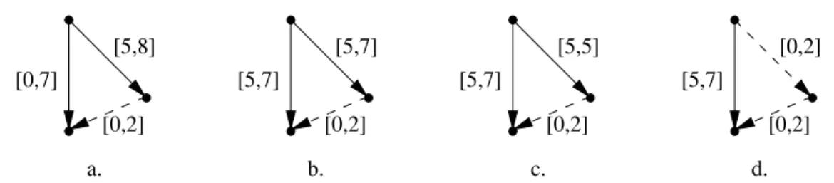
Figure 2 shows four STNU with the same nodes and edges, but with different labels and properties (uncontrollable edges are represented by dashed arrows).

4.2 Interfacing STNU with simple games

In order to be a strategy for a simple game G, an STNU shall speak about the transitions of the TTGA A done before reaching some goal state in G. We formalize here this relation by defining (1) the interface of a gameGand (2) the satisfaction relation between an STNU and a game interface.

Intuitively, the interface of a simple game is an STNU containing a time- point for each transition of the game that can take place until the horizon of the game is reached; these time-points are related with edges labeled by the timing

(10)

[5,7] [5,7] [5,7]

[0,2]

[0,7]

a.

[0,2]

b.

[0,2]

c.

[0,2]

d.

[5,5]

[5,7]

[5,8] [0,2]

Fig. 2.STNU (a) DC but not reduced, (b) reduced wrt shortest path, (c) reduced wrt DC, (d) not DC.

constraints in the TTGA of the game. For tasks with cycles, a transition may appear several times until the game end. Due to the special form of tasks, we can unfold these tasks and compute (see Appendix B for details) for each transition m of a task i its maximal number of occurrence in the horizon B, denoted by µ(i)(m)≥0. Thus, we can identify each transitionethat can be executed during the game horizon by a triple (i, m, u) where i ∈ I is the identifier of the task owninge,m∈L_iis the source location ofe, andu∈[1, µ(i)(m)] is the occurrence number computed fore. In the following, we denote byprec(i, m, u) the transition preceding (i, m, u) in the unfolding of taski. Similarly,prec_c(i, m, u) denotes the last controllable transition before (i, m, u) in the unfolding of task i. If no such preceding transition exists, both notations return (i,0,1).

The interface of a simple game G with horizon B is an STNU ZG = hNG, EG, CG, lG, uGiand a labeling of time-pointsσG:I×N×N→NGdefined as follows:

– NG contains two special time-points t0 and tG corresponding respectively to the initial moment and to the goal moment. These two time-points are related by an edge (t0, tG)∈CG labeled by [0, B] to model the finite horizon constraint of the game. Since the time-pointt₀is the initial moment on all tasks, it is labeled by (i,0,1) for anyi∈I.

– For each taskiand each transitionmofi,N_Gcontains a number of time-points given byµ(i)(m).

– E_G relates the nodes in N_G wrt timing constraints and ordering of transitions in A. For example, a transition e = m 7→ (gd, gx, a, n) in some task i defines inE_G a first set of edges{prec_c(i, m, u)−−−→(i, m, u)^I^gx |1≤u≤µ(i)(m)}

where Ig_x is the interval on the local clock defined bygx. This set is included in CG iff a = c; it models the timing constraint gx which defines a delay from the last reset of the local clock. The second set of edges defined by e is {(i, m, u)−−−−−→(i, n, u)^[0,+∞) |1 ≤u≤µ(i)(m)} ⊂C_G and it models the ordering of transitions starting frommandnin taski.

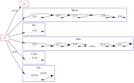
Example 3. Figure 3 gives the interface of the game considered in Example 2.

The time-points are put in clusters recalling the task owning the transitions represented by these time-points. Controllable edges without labeling intervals are implicitly labeled by [0,+∞).

The interface is the “largest” STNU for Gwrt the time-points represented and the constraints on edges, but it can not represent a strategy for Gbecause

(11)

Move

Pic

Arm

Com

Vw t0

tG [0,14]

[0,0]

[3,4] [5,6] [1,2] [3,4] [5,6]

[3,6]

[2,4] [1,3] [2,4]

..3 times... [1,3] [2,4]

[8,10]

[20,30] [40,50]

Fig. 3.Interface for the Explorer game with horizonB= 14.

neither goal nor safety constraints are satisfied. In fact, the interface is used as a sanity check for candidate STNU strategy: a candidate strategy shall contain a “consistent” subset of time-points and edges in the interface ofG. Formally, an STNUZ =hN, E, C, l, uiis said tosatisfy the interface (ZG, σG) of a game G, denoted by Z |= G, iff (1)N contains t0 and tG, (2) N contains a subset of NG closed by the precedence relation, i.e., if the time-point (i, m, u) is inN then all its predecessors in the unfolding ofiare also present, and (3) the edges defined inEGbetween the nodes inN are also defined inE with the same kind (controllable or uncontrollable) and the same labeling intervals for uncontrollable edges; for controllable edges, the labeling interval in Z shall be included in the corresponding one in ZG. Intuitively, Z satisfies the interface of the game Gif it puts exactly the same constraints asZG on common uncontrollable edges and it may squeeze the constraints on controllable edges.

5 Computing STNU Strategies

We consider the following two problems for simple gamesGwith horizonBgiven in unary:

G-Solve: Decide if a winning strategy exists for G.

G-Solve-STNU: Decide if a winning STNU strategy exists forG.

(12)

Our first result is that, despite the simplicity of the game considered, the problem of finding strategies for such games is still NP-hard.

Theorem 1. The G-Solve problem is NP-hard.

Proof. The proof consists in reducing the CliqueCover problem [12] to the synthesis of a strategy for simple games. An instance of the CliqueCover problem is an integer k and an undirected graph P = (V, E) with n vertices (|V|=n) numbered 1 ton. TheCliqueCoverproblem is to decide whether a graph can be partitioned intokcliques. We explain how to reduce this problem to G_k-Solve problem, whereG_k is a simple game. The TTGA ofG_k is built as follows: for each vertexi∈[1, n] ofP, we define a task indexed byiwith the form:

1−−−−−−−−→^xⁱ^≥0,c,{xⁱ^} 2−−−−−−−−−→^0≤xⁱ^<1,u,{} 3. The setSofGkis specified byV

(i,j)6∈Ei@2] j@2, i.e., for each pair of vertices (i, j) such that there is no edge inEbetweeniandj we ask mutual exclusion between the locations 2 of the corresponding tasks. The setGofG_kis specified by∧ii@3, i.e., all tasks shall reach location 3. The horizon ofG_k is fixed tok. It follows (details in Appendix C) thatP can be covered by k cliques or less iff the instance of theG_k-Solve problem has a strategy to win.

Moreover, an STNU strategy can be built forGk. A direct consequence of the proof above is:

Corollary 1. The G-Solve-STNU problem is NP-hard.

The upper bound of complexity forG-Solve is given by the upper bound of solving reachability game problems for TGA, i.e., EXPTIME in [15]. This tight upper bound is obtained for general TGA with safety games and state based (memory less) strategies.

The following theorem says that this upper bound decreases for G-Solve- STNU problems to NP.

Theorem 2. The G-Solve-STNU problem is NP-complete.

Proof idea. We show that it exists a correct and complete polynomial test to check that an STNU strategyZ satisfying the interface of a simple gameGis a winning STNU strategy. Then, the theorem follows since for a horizon B given in unary, the description of a candidate STNU strategy is polynomial in the number of transitions inGand in the horizonB (Lemma 5).

The polynomial test is given on Figure 4. First (line 1), Z is filled with the missing time-points and edges in the interface of G thus obtaining a new STNUZ. Second (line 2), the DC algorithm is applied onZ to test its dynamic controllability and to compute its reduced form. Third (line 6), Zb is tested for satisfaction of goal and safety constraints inG. This test is done by searching inZb a set of edges (calledshapes) for each goal constraint inG, for each discrete guard on controllable transitions of the TTGA ofG, and for each safety constraint in S.

The technical point in the proof is the definition of shapes such that the test is correct and complete. A shape is a positive boolean composition of precedence

(13)

Require: STNUZ s.t.Z |=G.

Ensure: Returns true ifZ is a winning strategy forG.

1: Z←Z∪ZG

2: Zb←ΠDC(Z) 3: if Zb=⊥then 4: returnfalse 5: end if

6: returnZb|=shape_Goal andZb|=shape_Safe

Fig. 4.Test for winning STNU strategy.

relations between two time-points. A time-pointt precedes the time-point t⁰ in an STNUZ, denoted by Z `t≺t⁰, iff Z contains an edge fromt to t⁰ labeled by an interval included in (0,+∞). For example, the shape used to test that the goal constraint i@[m, n] is satisfied by Zb is prec(i, m, u) ≺t_G∧t_G ≺(i, n, u) (see Figure 7). The test succeeds if such shape exists in Zb for some u. To test

tG prec(i,m,u)

(i,n,u) i

Fig. 5.Shape for goal constrainti@[m, n].

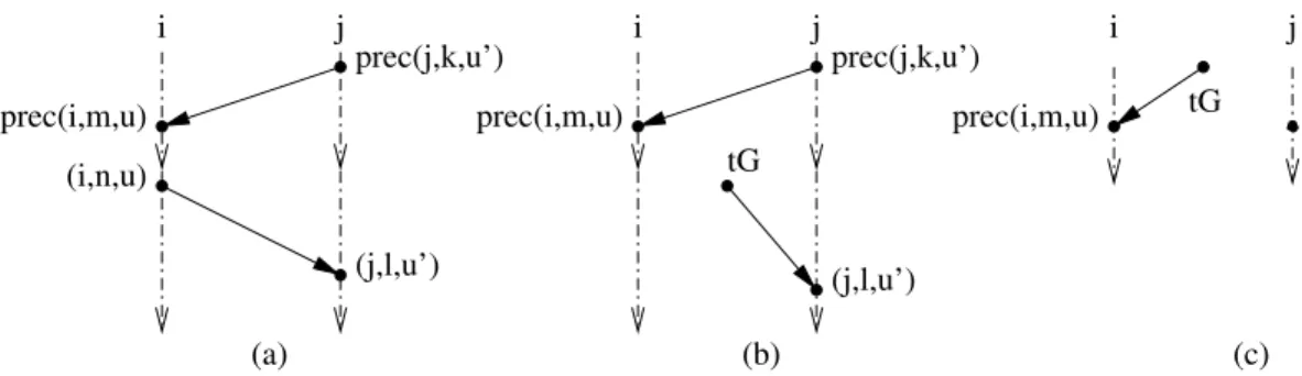
safety constraint and discrete guards on transitions, the shapes shall be carefully defined in order to obtain completeness. For example, the shape for a constraint i@[m, n] =⇒j@[k, l] is the disjunction of three cases which are not disjoint (see Figure 8). Intuitively, the constraint is satisfied if for any occurrenceuof transitions in taskileading to locationm(time-pointprec(i, m, u)) and leaving the locationn(time-point (i, n, u)) there exists an occurrenceu⁰ of the transition in taskj leading to locationk(time-pointprec(j, k, u⁰)) and leaving the locationl (time-point (j, l, u⁰)) such that one of the following cases holds:

(i) the safety constraint is entirely satisfied since prec(j, k, u⁰) precedes prec(i, m, u) and (i, n, u) precedes (j, l, u⁰),

(ii) the safety constraint is satisfied at the beginning of the interval [m, n] for i but nothing is asked for the end because the goal (time-pointtG) is reached before the end of the intervalj@[k, l]; indeed, the game semantics asks that safety constraints are satisfied until the goal is reached but not beyond,

(iii) the safety constraint is not satisfied because the considered time-points are after the goal.

The correctness proof follows easily from the definition of shapes. The completeness is based on the convexity of the STNU strategies and the fact that the

(14)

(a) (b) (c) tG

prec(i,m,u) prec(j,k,u’)

i j i j i j

prec(i,m,u)

prec(j,k,u’)

(j,l,u’) (i,n,u)

prec(i,m,u)

(j,l,u’)

tG

Fig. 6.Shape for safety constrainti@[m, n] =⇒j@[k, l].

shapes defined can not exclude correct but convex STNU. The full proof is given in Appendix D.

To finish the proof, we compute the complexity of the proposed algorithm.

If the horizonB is given in unary, the number of points in the interface ofGis polynomial, so the first two steps of the algorithm (lines 1–2) are also polynomial (DC is polynomial in the number of time-points in ˜Z). Testing shapes (line 5) is also polynomial. Indeed, to test the satisfaction of some constraint (in guards, goal, or safety), one has to find a set of edges of constant size (the shape) in the STNU. But the number of edges in STNU is quadratic wrt the number of nodes, so we obtain the following result:

Lemma 1. Given an STNUZ satisfying the interface of a gameG, the problem of deciding ifZ is a winning strategy forGis in PTIME.

Now, let us compute the size of a representation for STNU that are candidate strategies for a game G. If the TTGA of G has n transitions, the maximal number of time-points in the interface of G is n×B+ 2, limit reached when each transition takes one time unit. Then, the maximal number of edges that has to be specified for the STNU candidate isO(n²×B²). Each of these edges is labeled by an interval given by two integer numbers. However, these numbers are limited by the horizonB.

Lemma 2. The size of describing a candidate STNU strategy for a game Gis O(n²×B³)wherenis the number of transitions in the networkN andB is the horizon of the game.

6 Algorithm for solving simple games

The proof of Theorem 2 gives also the sufficient conditions for an STNU to be a winning strategy for a simple gameG: (1) it has to satisfy the interface ofG, (2) it has to be DC, and (3) its reduced form byΠ_DC has to implement some precedence relations (i.e., some shape) for each time-point concerned by a guard, goal, or safety constraint. The last condition defines a combinatorial space W for building winning STNU strategies: each strategy represents a choice of the

(15)

shapes implementing the constraints ofGfor each time-point in the interface of G.

Therefore, we propose a fully forward algorithm for building winning STNU strategy, called in the following Win STNU, which does a backtracking search in the combinatorial spaceW. The algorithm starts with the STNU interface of G,ZG (see Section 4.2). For each choice step in W, it builds a partial solution by adding to ZG the controllable edges given by the shape chosen. The algorithm may useΠDC as a selection (cut off) test for the partially built solutions.

Otherwise, when all choices are done,ΠDC is applied to test the DC property of the solution built.

Win STNU does not find all winning strategies of G but only “standard”

ones, i.e., STNU strategies which contain all the time-points of the interface and have maximal intervals on controllable transitions (see Appendix E). Moreover, the number of time-points of a solution is bounded by B times the number of transitions inG. The properties of our algorithm are summarized by the following proposition which proof is given in Appendix E.

Proposition 1. The algorithmWin STNUis correct and complete wrt standard STNU strategies. It builds solutions of size (number of nodes and edges) quadratic in the size of the game.

7 Conclusion

We define a class of timed games for which searching winning strategies in STNU form is NP-complete. As a corollary, we obtain a fully forward algorithm for solving the finite horizon reachability timed games. This algorithm builds STNU strategies which are finite memory strategies with no discrete choices but including several orderings between independent actions of the controller. Moreover, the size of these strategies is small, i.e., quadratic in the size of the game. Fur- ther works focus on providing a good implementation of our algorithm and on comparing the strategies obtained using other criteria, e.g., their volume [5].

References

1. Y. Abdedda¨ım, E. Asarin, M. Gallien, F. Ingrand, C. Lessire, and M. Sighire- anu. Planning Robust Temporal Plans A Comparison Between CBTP and TGA Approaches. InICAPS. AAAI, 2007.

2. Y. Abdedda¨ım, E. Asarin, and O. Maler. On optimal scheduling under uncertainty.

InTACAS, volume 2619 ofLNCS, pages 240–253. Springer-Verlag, 2003.

3. Y. Abdedda¨ım, E. Asarin, and O. Maler. Scheduling with timed automata.Theor.

Comput. Sci., 354(2), 2006.

4. M. Ai-Chang, J. Bresina, L. Charest, A. J´onsson, J. Hsu, B. Kanefsky, P. Maldague, P. Morris, K. Rajan, and J. Yglesias. MAPGEN: Mixed initiative planning and scheduling for the Mars 03 MER mission. InISAIRAS, 2003.

5. E. Asarin and A. Degorre. Volume and entropy of regular timed languages. HAL preprint hal-00369812, 2009.

(16)

6. G. Behrmann, A. Cougnard, A. David, E. Fleury, K. Larsen, and D. Lime. Uppaal- Tiga: Time for playing games! In CAV, volume 4590 ofLNCS. Springer-Verlag, 2007.

7. J. Bengtsson, B. Jonsson, J. Lilius, and W. Yi. Partial order reductions for timed systems. In CONCUR, volume 1466 of LNCS, pages 485–500. Springer-Verlag, 1998.

8. F. Cassez, A. David, E. Fleury, K. Larsen, and D. Lime. Efficient on-the-fly algorithms for the analysis of timed games. In CONCUR, volume 3653 ofLNCS.

Springer-Verlag, 2005.

9. T.H. Cormen, C.E. Leiserson, and R.L. Rivest. Introduction to Algorithms. The MIT Press, 1997.

10. R. Dechter, I. Meiri, and J. Pearl. Temporal Constraint Network. Artificial Intel- ligence, 49(1-3):61–95, 1991.

11. A. Fehnker.Guiding and Cost-Optimality in Model Checking of Timed and Hybrid Systems. PhD thesis, KUNijmegen, 2002.

12. M.R. Garey and D.S. Johnson. Computers and Intractability: A Guide to the Theory of NP-Completeness. W. H. Freeman, 1979.

13. M. Ghallab and H. Laruelle. Representation and control in IxTeT, a temporal planner. InAIPS, 1994.

14. E. Gr¨adel, W. Thomas, and T. Wilke, editors. Automata, Logics, and Infinite Games: A Guide to Current Research [outcome of a Dagstuhl seminar, February 2001], volume 2500 ofLNCS. Springer-Verlag, 2002.

15. T. Henzinger and P. Kopke. Discrete-time control for rectangular hybrid automata.

Theor. Comput. Sci., 221:369–392, 1999.

16. N. Laya¨ıda, L. Sabry-Isma¨ıl, and C. Roisin. Dealing with uncertain durations in synchronized multimedia presentations. Multimedia Tools Appl., 18(3):213–231, 2002.

17. Solange Lemai and F. Ingrand. Interleaving temporal planning and execution in robotics domains. InAAAI, San Jose, CA, USA, 2004.

18. X. Liu and S. Smolka. Simple linear-time algorithms for minimal fixed points (extended abstract). InICALP, volume 1443 ofLNCS. Springer-Verlag, 1998.

19. D. Lugiez, P. Niebert, and S. Zennou. A partial order semantics approach to the clock explosion problem of timed automata. Theor. Comput. Sci., 345(1):27–59, 2005.

20. O. Maler, A. Pnueli, and J. Sifakis. On the synthesis of discrete controllers for timed systems. InSTACS, volume 900 ofLNCS. Springer-Verlag, 1995.

21. P. Morris. A structural characterization of temporal dynamic controllability. In CP, volume 4204 ofLNCS. Springer-Verlag, 2006.

22. P. Morris, N. Muscettola, and T. Vidal. Dynamic control of plans with temporal uncertainty. InIJCAI, 2001.

23. S. Tripakis and K. Altisen. On-the-fly controller synthesis for discrete and dense- time systems. InFM, volume 1706 ofLNCS. Springer-Verlag, 1999.

24. T. Vidal. A unified dynamic approach for dealing with temporal uncertainty and conditional planning. InICAPS, Breckenridge, CO, USA, 2000.

25. T. Vidal and H. Fargier. Handling contingency in temporal constraint networks:

from consistency to controllabilities. JETAI, 11(1), 1999.

(17)

A Semantics of TTGA

Astateof a taskTiis a triple (`, s, v)∈L×N^I×R^X≥0such thats[i] =`; (`, s) is called the discrete part of the state. From a state (`, s, v) such thatv |=tc[`]≺, a task can either let time progress or do a discrete transition and reach a new state. This is defined by the transition relation−→built as follows:

– For a = c, (`, s, v)−→(`^a ⁰, s⁰, v⁰) iff there exists a transition (`, gd, gx, a,{xi}, `⁰) ∈ Ei such that s |= gd, v |= gx, s⁰ = s[i@`⁰], v⁰ = v[{xi}], and v⁰ |= tc(`⁰)≺ (i.e., the upper bound of constraints in tc(`⁰)_≺).

– For a = u, (`, s, v)−→(`^a ⁰, s⁰, v) iff there exists a transition (`, true, gx, a,{xi}, `⁰)∈Ei such thatv|=gx, s⁰=s[i@`⁰], andv|=tc(`⁰)≺. – Forδ∈R≥0, (`, s, v)−→(`, s, v^δ ⁰) ifv⁰=v+δthenv⁰, v∈[[tc[`]_≺]].

Thus, the semantics of a task T_i is a labeled transition system (LTS) S_T_i = (Q, q₀,−→) whereQ=L×N^I ×R^X≥0, q₀ = (`⁰_i, s₁,0), and the set of labels is {c, u} ∪R≥0.

The semantics of TTGA is defined similarly. A state of the TTGA is a tuple (`, s, v) such that for any taski s[i] =`[i] andv|=∧_i∈Itc[`[i]]_≺. The transition relation −→ is defined as above for discrete transitions. For timed transitions, all timed constraints of transitions starting from`shall be verified: if δ∈R≥0, (`, s, v)−→(`, s, v^δ ⁰) ifv⁰=v+δ, andv⁰, v∈[[∧_i∈Itc[`[i]]_≺]].

Arun of a TTGA is a sequence of alternating time and discrete transitions in its LTS. Runs can also be represented by timed words (a₁, τ₁). . .(a_m, τ_m) where a₁, . . . , a_m ∈ Act and τ₁, . . . , τ_m are the real values corresponding to the time at which each discrete action is executed. Then, a normal run has a timed word such that when i ≤j then τi ≤τj. We denote by last(ρ) the last state of a run ρ. We denote by Runs(N,(`, s, v)) the set of normal runs of a networkN starting in state (`, s, v). Amaximal run is a run where time is not blocked by the time constraints, i.e., either it is an infinite run or it ends in a state which location has no discrete successor by anyEi or in a state such that s6|=guard(`) for any` of the state. The constraint (iv) of the definition gives a necessary syntactic condition on the timed constraints of transitions in order to obtain complete runs. Indeed, it implies that for any two successive transitions of a task Ti, `−−−−−−→^ψ¹^,ϕ¹^,a¹ `⁰−−−−−−→^ψ²^,ϕ²^,a² `⁰⁰ such that a1 6= c we have that if, e.g., ϕ1 =xi ∈ [m1, M1] and ϕ2 =xi ∈ [m2, M2] then M1 < m2 ≤ M2. Then, by firing the first transition we are sure that the state invariant of`⁰ is satisfied.

B Computing Unfolding of Tasks

Due to the form of TTGA, the minimum execution time of each TTGA is given by the following formula:

δ(Ti)(ω) =δ1(Ti) +ω×δ_∗(Ti)

(18)

whereδ₁(T_i) is the minimum time taken to execute the first time all transitions of the task T_i, ω is the number of iterations of the loop ofT_i, and δ_∗(T_i) is the minimum time taken to execute the next iterations of the loop ofT_i. All these times are computed only from the timed constraints on the transitions of Ti

and the computation does not consider the dependences implied by the discrete guards of transitions.

The minimum execution time for the first execution of all transitions ofTi is given by:

δ₁(T_i) =Σ_{t ctrl.}δ₁(t) +δb₁(T_i)

δ1(t) =max({l[t]} ∪ {l[t−1]|(t−1) unctrl}) δb₁(T_i) =

0, Ei(|Li| −1)ctrl.

l[|Li| −1], Ei(|Li| −1)unctrl.

wherel[t] is the lower bound (stronger constraintc≤xi) in the timed guard of transition t. Intuitively, the minimum time for the first execution of Ti is computed from the lower bounds given by the time constraints on the controllable and uncontrollable transitions ofTi. Recall that transitions are indexed by their source locations, so t−1 represent the transition beforet in the TTGA. Also, since controllable transitions reset the local clock, the minimal execution time of the task is the sum of minimal times elapsed between two controllable transitions plus the residue due to the en of the task which may be not a controllable transition. The time elapsed between two successive controllable transitions t₁ and t₂ is given either by the maximum between the lower bound of t₂ and the lower bound of the uncontrollable transition just before t2, i.e., t2−1 if it is uncontrollable.

The minimum execution time of the second and next iterations of the loop of Ti is computed similarly by tacking the lower bounds of time constraints on the controllable transitions of the loop. However, when considering the predecessor of a controllable transition in the loopt, we have to stay in the loop, i.e.,t−1 has to be in the loop. Then, for the first controllable transition of the loop we have to consider the last uncontrollable transition in the loop (given by |Li|) if it exists:

δ_∗(Ti) =Σtctrl. in loop ofT_iδ_∗(t) +δb_∗(Ti)

δ∗(t) =max({l[t]}∪

{l[t−1]|t−1 is unctrl. in the loop}

δb_∗(T_i) =

0, |Li|is ctrl.

l[|L_i|],|L_i|is unctrl.

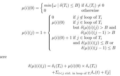
We define the mapping µ : I → N → N which gives for each transition j (j ≥ 1) of the task i the maximum number of unfolding in order to cover the horizon B. Moreover, µ(i)(0) returns the maximum number of complete

(19)

executions of the loop ofT_i to coverB.

µ(i)(0) =

min{ω|δ(T_i)≤B}ifδ_∗(T_i)6= 0

0 otherwise

µ(i)(j) = 1 +











0 ifj6∈loop ofT_i µ(i)(0) ifj∈loop ofTi

but δ(µ)(i)(j)> B and δ(µ)(i)(j−1)> B µ(i)(0) + 1 ifj∈loop ofTi

andδ(µ)(i)(j)≤B or δ(µ)(i)(j−1)≤B where

δ(µ)(i)(j) =δ₁(T_i) +µ(i)(0)×δ_∗(T_i) +Σt<jctrl. in loop ofTiδ∗(t) +l[j]

Example 4. The computation of unfoldings for the Explorer rover (see Figure 1) is given on Table 1. The table pictured in this figure gives for each task and for each transition (named by its source location) the number of time-points represented for this transition in the game interface.

Transitions (j) Task (i)µ(0)(i)δ(Ti)(ω) 1 2 3 4 5 6

Move 0 9 + 9ω 2 2 2 2 1 1

Pic 0 3 1 1 – – – –

Arm 3 3 + 3ω 5 5 5 4 – –

Com 0 8 1 1 – – – –

Vw 0 40 1 1 1 – – –

Table 1.Unfolding computation for Explore example.

C Proof of Theorem 1

Let k be an integer andP be an undirected graph P = (V, E) withn vertices (|V|=n) numbered 1 ton. Let G_k be the game built at Theorem 1. We show thatP can be covered bykcliques or less iff theG_k-Solve problem has a strategy to win.

(⇒) If P has at mostk cliques, let V =∪_{0≤`≤k−1}V_` with V_` the set of `^th clique. By definition ofG_k, for any`, all tasks indexed by vertices inV_` can be in their location 2 at the same time. Then, the first transition of these tasks can be executed at the same time without invalidating the safety property ofGk and they have to leave location 2 after one time unit at most. A winning strategy

(20)

forG_k is to take at momenttthe controllable transition of the tasks indexed by the vertices inV_t. By construction ofG_k, all tasks will end in location 3 before ktime units and the safety constraints are satisfied.

(⇐) If the gameGkhas a winning strategy, this strategy shall start all tasks in the interval [0, k]. Since each task takes at most one time unit, then there are at mostk groups of tasks executed simultaneously (i.e., in their location 1) during [0, k]. By construction ofG, these tasks correspond to vertices related by an edge inP, soP has at mostkcliques.

D Proof of Theorem 2

The proof gives a polynomial test to decide if an STNU strategyZsatisfying the interface of a simple gameGis a winning strategy forG(Lemma 3 and 4 below).

Then, the theorem follows since for a horizonB given in unary, the description of potential STNU candidate for a winning strategy is polynomial in the size of the game and the boundB (Lemma 5 below).

The algorithm testing when an STNU is a winning strategy for a simple game is given on Figure 4.

The shapes used in the test algorithm are defined from the goalG, the guards in the networkN, and the safety constraintsS.

Anatomic shapeis a precedence constraint between two time-points, denoted by t ≺ t⁰, saying that the time-point t precedes time-point t⁰. An STNU Z containing the time-pointst andt⁰ satisfies the atomic shapet≺t⁰, denoted by Z `t≺t⁰, iffZcontains a link fromttot⁰whose label is an interval with strictly positive lower bound (i.e., an interval in (0,+∞)). Atomic shape constraints are combined using conjunctions, disjunctions and quantification over time-points to form shape constraints.

More precisely, the time-points in shape constraints belong to STNU satisfying the interface ofG, so they are labeled (due toσ⁻¹_G ) by triples (i, m, u) with i∈I the index of the task, m≥1 the order number of the state source of the transition, andu≥1 the occurrence of the transition. Quantification in shapes is done over the occurrence numbersuin time-points labels.

Shapes (without quantification) can be represented graphically as shown on Figures 7 and 8. Time-points are labeled by their tuple (tasks index, transition index, occurrence number). Dashed lines are used to show time-points belonging to the same task.

Formally, the syntax ofshape constraints is:

Atomic shape3a::= (i, m, u)∼t_G|(i, m, u)∼(j, k, l) Shape3s::=a|s∧s|s∨s| ∃u. s| ∀u. s

where i, j ∈ I, m, k ≥ 1 are index of transitions in T_i resp. T_j, u, l ≥ 1 are occurrences of these transitions, and∼∈ {≺,}.

For example, the shape constraint of Figure 7 isprec(i, m, u)≺tG∧(i, n, u) tGwhere we useprec(i, m, u) to represent the time-point for the transition preceding the transition (i, m, u) onTi.

(21)

tG prec(i,m,u)

(i,n,u) i

Fig. 7.Shape fori@[m, n]∈ G.

The shape constraints used in the algorithm to test the goal are built from the goal constraints as follows:

shape_Goal ::= ^

i@[m,n]∈G

∃u. prec(i, m, u)≺tG∧tG≺(i, n, u)

which means that for each constraint in the goal, γ=i@[m, n], there exists an occurrence number for the transitions preceding transition (i, m) (which leads to the m^th state of Ti) and the transition (j, n) (which goes out from the n^th state ofTi) such that the goal is reached attG between these two moments.

Shapes used to test safety are generated from safety constraints as follows:

shape_Safe ::=^

i∈I





^

act[(i,m)]∈Act_c

shape_(i,m)



∧ ^

δ∈S

shape_δ

where the first set of conjuncts gives shape constraints from the guards of controllable transitions in each TTGA, while the second set represents shapes from the safety constraintsS ofG. In defining these shapes, a special treatment shall be considered for points succeeding the goal time-point tG because the safety constraints shall be satisfied until reaching the goal but they are not mandatory afterwards.

Consider now a controllable transition (i, m) and some of its occurrence u.

Then, the safety constraint corresponding to the guard of (i, m) may be ignored if time-point corresponding to (i, m, u) is after the goal. Otherwise, for each indexed interval constraintj@[k, l] in the guard of (i, m), the time-point (i, m, u) shall be between some occurrenceu⁰ of the transition leading to the statekofTj

(i.e.,prec(j, k, u⁰)) and the transition going out from the statel. Then,shape_(i,m) is defined by:

∀u. t_G≺(i, m, u)∨ V

j@[k,l]∈guard[(i,m)] ∃u⁰. prec(j, k, u⁰)≺(i, m, u)

∧(i, m, u)≺(j, l, u⁰)

The shapes for safety constraints ini@[m, n] =⇒j@[k, l] are generalization of shapes for guards:

∀u. tG≺prec(i, m, u)∨

∃u⁰. prec(j, k, u⁰)≺prec(i, m, u)∧ (i, n, u)≺(j, l, u⁰) ∨ tG≺(j, l, u⁰)

(22)

Intuitively, the i^th TTGA is between states m and n while the j^th TTGA is between states kandl if for any occurrenceuof transitions leading to state m (prec(i, m, u)) and the one leaving the state n((i, n, u)) there exists an occurrence u⁰ of transitions of Tj leading to state k (prec(j, k, u⁰)) and leaving the statel((j, l, u⁰)) such that one of the following cases is true:

– the safety constraint is entirely satisfied by theuoccurrence of the execution ofTi between statesm andn and by the u⁰ occurrence of the execution of Tj between stateskandl,

– the safety constraint is satisfied at the beginning of these executions but not at the end of the intervals due to the fact that the goal is reached before execution ofTj betweenkandl ends, or

– the safety constraint is not satisfied because the considered occurrences are after the goal.

Figure 8 gives an illustration of each case above. Note that the above cases are not disjoint and this is an important fact for the proof of completeness of our test procedure (Lemma 1).

(a) (b) (c)

tG

prec(i,m,u) prec(j,k,u’)

i j i j i j

prec(i,m,u)

prec(j,k,u’)

(j,l,u’) (i,n,u)

prec(i,m,u)

(j,l,u’)

tG

Fig. 8.Shape for safetyi@[m, n] =⇒j@[k, l] ofS.

Finally, the shapes for mutual exclusion safety constraintsi@[m, n]] j@[k, l]

are defined as follows:

∀u. tG≺prec(i, m, u)

∨∃u⁰. (j, l, u⁰−1)≺prec(i, m, u)

∧(i, n, u)≺prec(j, k, u⁰)

∧ ∀u. tG≺prec(j, k, u)

∨∃u⁰. (i, n, u⁰−1)≺prec(j, k, u)

∧(j, l, u)≺prec(i, m, u⁰)

where for any i ∈ I and any state m in T_i, (i, m,0) represents t₀. Intuitively, the safety constrainti@[m, n]] j@[k, l] is satisfied if for each occurrenceuof an execution between statesmandninTi (andkandl inTj) one of the following conditions holds:

(23)

– this occurrence is after the goal, i.e., theuoccurrence of the transition leading to them(resp.k) is after the goal, or

– the execution takes place strictly between occurrencesu⁰−1 andu⁰ of execution ofTj from statekto l(resp.Ti from statemton) for someu⁰≥1.

Like for inclusion constraints, these two cases are also overlapping.

The following lemma states the correctness and the completeness of our algorithm.

Lemma 3. An STNUZ satisfying the interface of a gameGis a winning strategy iff the algorithm IsWinningStrategyreturns true.

Proof. (⇐) LetZ be an STNU such thatZ`Gand the test algorithm returns true. The algorithm builds from Z an STNU which is DC and satisfies all the goal and safety constraints. By definition of winning strategies, the result follows.

(⇒) The proof of completeness uses the convexity of the STNU strategies and the fact that the shape tested cannot exclude correct but convex STNU.

LetZ be a winning strategy satisfying the interface ofG. ThenZ is already DC and satisfies the goal and safety constraints.We suppose thatZis in the reduced form of DC.

The algorithm first completes Z to obtain the full interface of G. However, the time-points added are only appended to the last time-point of each task so they can not influence the links inZ. Then, the DC algorithm applied to ˜Z only introduces more controllable links involving the newly introduced time-points, but does not change the original part ofZ.

Then, sinceZ is contained in Zb and it is a winning strategy, it means that each schedule of Z determines a play which goes through a goal configuration.

Since (1) STNU can not represent union of goal states and (2) the constraints on states inGare disjoint imply that only one possibility to satisfy state constraints in Gis present inZ. This configuration can be used to satisfy the shape for the goal.

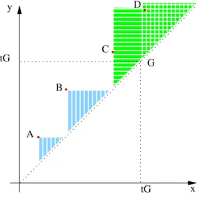
All plays ofZalready satisfy the safety constraints (guards and constraints in S). Since the added points in ˜Z are all after the goal configuration, they trivially satisfy the safety shapes since all these shapes are trivial for points aftertG. For time-points beforetG, we claim that these time-points satisfy exactly one of the disjunction of the shapes in shape_Safe. The idea is to show that (1) the shapes considered correspond to disjoint set of plays and (2) the plays of Z cannot be in two such shapes due to convexity ofZ.

Figure 9 gives an intuition of the point (1) for the shapes corresponding to inclusion safety constraints i@[m, n] ⇒ j@[k, l]. The plan represents in x axis the beginning of executions (prec(i, m, u) and prec(j, k, u⁰)) and in the y axis the end of theses executions ((i, n, u) and (j, l, u⁰)). Then all considered points shall be in the second half of the first quadrant. Points A, B, C and D represent occurrences of the executions in T_j respectively, i.e., the the first, second, third, and fourth occurrences ofprec(j, k, u⁰) and (j, l, u⁰). In fact, these points are DBM zones in Z, but they can be abstracted to points dues to the following property: the consecutive occurrences of executions of Tj are disjoint

(24)

and moreover, (j, l, u⁰) ≺ prec(j, k, u+ 1). The zones attached to pointsA–C andGcorrespond to executions onT_iallowed by the shape for safety constraint i@[m, n]⇒j@[k, l]. For points A and B situated before the goal (x andy are less thantG), the executions onTi shall satisfyprec(j, k, u⁰)≺prec(i, m, u) and (i, n, u) ≺ (j, l, u⁰). For point C, although the beginning of execution ofTj is beforetG, this execution ends after tG, so the executions allowed for Ti satisfy prec(j, k, u⁰) ≺ prec(i, m, u). Finally, all points greater thantG correspond to valid executions. It is important to see that we have only convex regions and any DBM covering these regions is fully included in one of them.

tG tG

y

x A

B

C D

G

Fig. 9.Proof of completeness.

If Z is winning, it shall satisfy every safety constraint δ of the form i@[m, n] =⇒ j@[k, l], that is for every moment t, if i is in t between states mandn, then eithertis aftertG or taskj is between statesk andl. The intervals in which j is between states k andl are disjoint (they are the hypotenuse of the triangle determined by the point attached to this point) because they correspond to different occurrences of this interval. Then, to satisfy the safety constraintδ, the hypotenuse for intervalsi@[m, n] shall be contained in the hypotenuse of triangles for points A–C or aftertG. These zone are those defined by the safety shape for this constraint.

To finish the proof, we compute the complexity of the proposed algorithm.

IfB (the game horizon) is given in unary, the number of points in the interface of G is polynomial, so the first two steps of the algorithm (lines 1–2) are also polynomial (DC is polynomial in the number of time-points in ˜Z). Testing shapes (lines 5 and 7) is also polynomial. Indeed, for each constraint (in guards, goal or safety), to test its satisfaction one has to find a (small) set of links in the graph defined by the STNU. The number of links in this graph is quadratic wrt the

(25)

number of vertices. We obtain then the following lemma which is a first step in establishing the complexity of our problem.

Lemma 4. Given an STNUZ satisfying the interface of a gameG, the problem of deciding ifZ is a winning strategy forGis in PTIME.

Now, let us compute the size of a representation for STNU that are candidate strategies for a gameG. If the TTGA ofGhasntransitions, the maximal number of time-points in the interface ofGisn×B+2, limit reached when each transition takes one time unit. Then, the maximal number of edges that has to be specified for the STNU candidate is O(n²×B²). Each of these edges is labeled by an interval given by two integer numbers which are limited by the horizonB. Then, we obtain the following result which finishes the proof of NP completeness.

Lemma 5. The size needed for describing a candidate STNU strategy for a game GisO(n²×B³)wherenis the number of transitions in the TTGA ofGandB is the horizon of the game given in unary.

E Properties of the simple algorithm

Proposition 2. All controllable edges in a SWS for a gameGare maximal wrt the game interface and constraints.

An STNU Z is included in some SWS iff (1)Z contains all time-points of the interface of G, (2) Z it is minimized using DC (so consistent), and (3) all controllable edges inZ are labelled by intervals included in the interval labeling the same edge in SWS.

Corollary 2. An STNUZ satisfying the interface ofGis a winning strategy iff Zb is included in some standard solution for the gameG.

where Zb is built as shown in Figure 4, i.e., by adding toZ all time-points and edges in the interface ofGand then applying DC.

Proof. ⇒If Z is a winning strategy forG, then it satisfies the goal and safety constraints in G and for any choice of the environment. Zb is obtained from Z by adding time-points which are not useful for satisfying safety and goal (since these time-points are related only with the last time-points ofZ on each task...).

Moreover, the DC algorithm does not change the controllability property. From the completeness result of Lemma 3, it results that in order to satisfy the goal and safety constraints of G, Z (and so Z) shall include some combination ofb safety and goal shapes. This combination gives the SWS to be chosen. But SWS is the maximal STNU with interface of G implementing the shapes and being controllable, soZb shall be included in this SWS.

⇐By the correctness of result of Lemma 3.

A direct consequence of the above property is given in the following corollary and it will be used to prove the relative completeness of our algorithm for solving simple games: