HAL Id: hal-01198948
https://hal.archives-ouvertes.fr/hal-01198948
Submitted on 14 Sep 2015
HAL is a multi-disciplinary open access archive for the deposit and dissemination of sci- entific research documents, whether they are pub- lished or not. The documents may come from teaching and research institutions in France or abroad, or from public or private research centers.
L’archive ouverte pluridisciplinaire HAL, est destinée au dépôt et à la diffusion de documents scientifiques de niveau recherche, publiés ou non, émanant des établissements d’enseignement et de recherche français ou étrangers, des laboratoires publics ou privés.
Simple Approximations of Semialgebraic Sets and their Applications to Control
Fabrizio Dabbene, Didier Henrion, Constantino Lagoa
To cite this version:
Fabrizio Dabbene, Didier Henrion, Constantino Lagoa. Simple Approximations of Semialgebraic Sets and their Applications to Control. Automatica, Elsevier, 2017, 78, pp.110-118. �hal-01198948�
Simple Approximations of Semialgebraic Sets and their Applications to Control
Fabrizio Dabbene
1Didier Henrion
2,3,4Constantino Lagoa
5September 14, 2015
Abstract
Many uncertainty sets encountered in control systems analysis and design can be expressed in terms of semialgebraic sets, that is as the intersection of sets described by means of polynomial inequalities. Important examples are for instance the solu- tion set of linear matrix inequalities or the Schur/Hurwitz stability domains. These sets often have very complicated shapes (non-convex, and even non-connected), which renders very difficult their manipulation. It is therefore of considerable im- portance to find simple-enough approximations of these sets, able to capture their main characteristics while maintaining a low level of complexity. For these reasons, in the past years several convex approximations, based for instance on hyperrect- angles, polytopes, or ellipsoids have been proposed.
In this work, we move a step further, and propose possibly non-convex approx- imations, based on a small volume polynomial superlevel set of a single positive polynomial of given degree. We show how these sets can be easily approximated by minimizing the L1 norm of the polynomial over the semialgebraic set, subject to positivity constraints. Intuitively, this corresponds to the trace minimization heuristic commonly encounter in minimum volume ellipsoid problems. From a com- putational viewpoint, we design a hierarchy of linear matrix inequality problems to generate these approximations, and we provide theoretically rigorous convergence results, in the sense that the hierarchy of outer approximations converges in volume (or, equivalently, almost everywhere and almost uniformly) to the original set.
Two main applications of the proposed approach are considered. The first one aims at reconstruction/approximation of sets from a finite number of samples. In the second one, we show how the concept of polynomial superlevel set can be used to generate samples uniformly distributed on a given semialgebraic set. The efficiency of the proposed approach is demonstrated by different numerical examples.
Keywords: Semialgebraic set, Linear matrix inequalities, Approximation, Sampling
1CNR-IEIIT; c/o Politecnico di Torino; C.so Duca degli Abruzzi 24, Torino; Italy
2CNRS; LAAS; 7 avenue du colonel Roche, F-31400 Toulouse; France.
3Universit´e de Toulouse; LAAS; F-31400 Toulouse; France.
4Faculty of Electrical Engineering, Czech Technical University in Prague, Technick´a 2, CZ-16626 Prague, Czech Republic.
5Electrical Engineering Department, The Pennsylvania State University, University Park, PA 16802, USA.
1 Introduction
In this paper, we address the problem of how to determine “simple” approximations of semialgebraic sets in Euclidean space, and we show how these approximations can be exploited to address several problems of interest in systems and control. To be more precise, given a set
K .
={x∈Rn:gi(x)≥0, i= 1,2, . . . , m} (1) which is compact, with non-empty interior and described by given real multivariate poly- nomialsgi(x), i= 1,2, . . . , m, and a compact setB ⊃ K, we aim at determining a so-called polynomial superlevel set (PSS)
U(p) .
={x∈ B:p(x)≥1}. (2)
that constitutes a good outer approximation of the setKof interest and converges strongly toK when increasing the degree of the real multivariate polynomialp to be found.
In particular, the proposed PSS is based on an easily computable polynomial approxi- mation of the indicator function of the set K. In the paper, we show that suitable ap- proximations of the indicator function can be obtained by solving a convex optimization problem whose constraints are linear matrix inequalities (LMIs) and that, as the degree of the approximation increases, one converges in L1-norm, almost uniformly and almost everywhere to the indicator function of the semialgebraic setKof interest. Moreover, the set approximations provided in this paper can be thought as a direct generalization of classical ellipsoidal set approximations, in the sense that if second degree approximations are used, we exactly recover well-known approaches.
The main motivation for the problem addressed in the paper is the fact that semialge- braic sets are frequently encountered in control. As an example, consider the Hurwitz or Schur stability regions of a polynomial. It is a well-known fact that the these regions are semialgebraic sets in the coefficient space. The polynomial inequalities that define these stability sets can be derived from well-known algebraic stability criteria. Another classical example of semialgebraic sets arising in control are LMI feasibility sets, also called spec- trahedra. Indeed, LMI sets are (convex) basic semialgebraic sets. To see this, consider the LMI set
KLMI .
={x∈Rn:F(x) =F0+F1x1+· · ·+Fnxn0}
where the matrix F(x) has size m×m, and observe that a vector x belongs to KLMI if and only if all the coefficients of the univariate polynomial
s7→det (sIm+F(x)) =g1(x) +g2(x)s+· · ·+gm(x)sm−1+sm
are nonnegative, i.e. xbelongs to the setK is defined in (1), where the polynomialsgi(x) are by construction sums of principal minors of the matrix F(x). The approach taken in this paper is the following: given the set K, we search for a minimum volume PSS that contains the set K. Since there is in general no analytic formula for the volume of a semialgebraic set, in terms of the coefficients of the polynomials defining the set1, it is
1See however reference [33] which explains how explicit formulas can be obtained with discriminants in exceptional cases.
very challenging to solve this optimization problem locally, let alone globally. Instead, the main contribution of this paper is to describe and justify analytically and geometrically a computationally tractable heuristic based on L1-norm or trace minimization. Second, we show that the same approach can be employed to obtain the largest (in terms of the L1 surrogate for the volume) PSS inscribed in K. Moreover, it is shown how the ideas put forth in this paper can be used to address two important problems: i) reconstruc- tion/approximation of a (possibly non-semialgebraic) set from samples belonging to it, and ii) uniform generation of samples distributed over a semialgebraic set. Examples of applications in a systems analysis and controller design context are also provided.
The work presented in this paper is an extension of the preliminary results in the con- ference papers [11] and [12], and it provides a more in depth analysis of both theoretical and implementation aspects. In particular, with respect to [11], the present manuscript contains more detailed proofs of the theoretical results, provides detailed algorithmic de- scriptions, and introduces inner PSS approximations. Similarly, the results on random sample generation of [12] are here described in more details, and an algorithm is pro- vided. Finally, all examples in the paper are new, and more control oriented applications are considered.
1.1 Previous work and related literature
The idea of approximating overly complicated sets by introducing simpler and easy man- ageable geometrical shapes is surely not new, it has a very long history, and it arises in different research fields such as optimization, system identification and control. In partic- ular, in the systems and control community, the most common approach is to introduce outer bounding sets, that is sets of minimum size which are guaranteed to contain the set to be approximated. For instance, in the context of robust filtering, set-theoretic state estimators for uncertain nonlinear dynamic systems have been proposed in [1, 18, 20, 39].
These strategies adopt a set-membership approach [19, 38], and construct (the smallest) compact set guaranteed to bound the system states that are consistent with the measured output and the norm-bounded uncertainty. The most common geometrical shape adopted in these work is the ellipsoidal one, for the double reason that it has a very simple descrip- tion – the center and the shape matrix are sufficient to provide a complete characterization – and that its determination usually can be formulated as a convex (usually quadratic) optimization problem. The use of ellipsoidal sets in the state estimation problems was introduced in the pioneering work [38] and used by many different authors from then on;
see, for example, [18, 20]. Outer approximation also arise in the context of robust fault detection problems (e.g., see [26]) and of reachability analysis of nonlinear and/or hybrid systems [25, 28]. Similarly,inner approximations are employed in nonlinear programming [34], in the solution of design centering problems [42] and for fixed-order controller design [24]. In this case, one aims at constructing the set largest size inscribed in the set of interest.
Besides ellipsoids, other shapes have been considered in the recent literature. The use of polyhedrons was proposed in [27] to obtain an increased estimation accuracy, while zonotopes have been also recently studied in [1, 21]. In [7] a heuristic based on polynomial
optimization and convex relaxations is proposed for computing small volume polytopic outer approximations of a compact semialgebraic set. More recent works, like for instance [5, 24, 32], employ sets defined by semialgebraic conditions. The closest approach to the one proposed in our paper can be found in [32], in which the authors use polynomial sum-of-squares (SOS) programming to address the problem of fitting given data with a convex polynomial, seen as a natural extension of quadratic polynomials and ellipsoids.
Convexity of the polynomial is ensured by enforcing that its Hessian is matrix SOS, and volume minimization is indirectly enforced by increasing the curvature of the polynomial.
In [5] the authors propose moment-based relaxations for the separation and covering problems with semialgebraic sets, thereby also extending the classical ellipsoidal sets used in data fitting problems.
Recently, the authors of [14] have proposed an approach based on randomization, which constructs convex approximations of generic nonconvex sets which are neither inner nor outer, but they enjoy some specific probabilistic properties. In this context, an approx- imation is considered to be reliable if it contains “most” of the points in the given set with prescribed high probability. The key tool in this framework is the generation of ran- dom samples inside the given set, and the construction of a convex set containing these samples.
1.2 The sequel
The paper is organized as follows. In Section 2 the notation used in this paper is intro- duced and the central problem addressed in this paper is defined. In order to be able to numerically solve the set approximation problem of interest, in Section 3 a related polynomial optimization problem is introduced and numerical methods for solving it are described in Section 4. In Section 5, we discuss how the results in this paper can be used to find inner approximations of semialgebraic sets. A first set of numerical exam- ples is provided in Section 6. Using the central results on set approximation mentioned above, in Section 7 we address the problem of reconstructing a set from a finite number of points in its interior. In Section 8 we provide algorithms for uniform sample generation in semialgebraic sets and in Section 9 some closing remarks are provided.
2 Problem statement
Before a description of the main problem addressed is provided, we introduce the basic notation that is used throughout the paper.
2.1 Notation
The notationA0 (0) means that the symmetric matrixAis positive definite (semidef- inite), and given two matrices A and B we write A B whenever A−B 0. Given a
setK ⊂Rn, its indicator function is defined as
IK(x) .
=
(1 if x∈ K
0 if x /∈ K (3)
and its volume or, more precisely, the Lebesgue measure of K, is denoted by volK .
= Z
K
dx= Z
Rn
IK(x)dx.
The set of all real coefficient polynomials of degree less than or equal to d is denoted by Pd. The monomial basis for this set is represented by the (column) vector πd ∈ Pd, so that any p∈Pd can be expressed in the following form
p(x) =πdT(x)p=πdd/2eT (x)P πdd/2e(x)
wherepis a real (column) vector2 andP is a symmetric matrix of appropriate size, often referred to as Gram matrix. Also, we denote by Σ2d the set of polynomials p∈ P2d that can be represented as sums of squares of other polynomials, i.e.
p=
np
X
k=1
p2k, pk ∈Pd, k = 1, . . . , np.
Finally, given a polynomial p∈Pd, define its L1 norm over a compact set B, denoted by L1B or just L1 when the set B used is clear from the context, as
kpk1
=. Z
B
p(x)dx.
2.2 Problem Statement
With the notation defined above, we are now ready to define the central problem in this paper. We consider the basic semialgebraic set K defined in (1), which is assumed to be compact and with a non-empty interior.
As discussed in the Introduction, the set K has typically a complex description in terms of its defining polynomials (e.g. coming from physical measurements and/or estimations).
For this reason, we aim at finding a “simpler” approximation of this set which has enough degrees of freedom to capture its characteristics. This approximation is the polynomial superlevel set (PSS)U(p) defined in (2) in terms of a real multivariate polynomialp∈Pd of given degree d. This degree controls the complexity of the approximation. Among the family of possible PSS that can be constructed, we search for the one that provides the setU(p) of minimum volume while containing the set of interestK, hence capturing most of its the geometric features. Formally, we define the following optimization problem
2Note that we use p to denote both the polynomial and the vector of its coefficients whenever no ambiguity is possible.
Problem 1 (Minimum volume outer PSS) Given d ∈ N and a compact semialge- braic setK, find a polynomialp∈Pd whose PSSU(p)is of minimum volume and contains K. That is, solve the following optimization problem
vd∗ .
= inf
p∈Pd volU(p)
s.t. K ⊆ U(p). (4)
Note that this problem can be viewed as the natural extension of the problem of computing the minimum volume ellipsoid containing K. Indeed, if K is convex and the polynomial p is quadratic (d = 2), then the infimum of problem (4) is attained, and the optimal set U(p) is given by the unique (convex) ellipsoid of minimum volume that containsK, called L¨owner-John ellipsoid. In particular, if K is the convex-hull of a finite set of points, this ellipsoid can be computed by convex optimization, see e.g. [4,§4.9].
We remark however that, for d greater than 2, the optimization problem (4) is nonlinear and semi-infinite, in the sense that the optimization is over the finite-dimensional vector spacePd, but subject to an infinite number of constraints, necessary to cope with the set inclusion.
Theorem 1 The sequence of infima of problem (4) monotically converges from above to volK, i.e. for all d≥1 it holds vd∗ ≥vd+1∗ and limd→∞v∗d= volK.
Proof: As in [23, Section 3.2], let x 7→ d(x,K) be the Euclidean distance to set K and with k >0 let K :={x ∈ B : d(x,K)< k} be an open bounded outer approximation ofK, so that B\Kk is closed with limk→∞k = 0. By Urysohn’s Lemma [37, Section 12.1]
there is a sequence of continuous functions (fk)k∈N with fk :B → [0,1] such that fk = 0 onB\Kk andfk= 1 onK. In particular, notice that volK ≤volU(fk)≤volK+ volKk\K and since limk→∞volKk\K= 0 it holds limk→∞volU(fk) = volK.
By the Stone-Weierstrass Theorem [37, Section 12.3] we can approximatefkuniformly on B by a sequence of polynomials (p0k,d)d∈N with p0k,d∈Pd, i.e. supx∈B|fk(x)−p0k,d(x)|< 0d with limd→∞0d = 0. Defining pk,d := p0k,d + 20d, the sequence of polynomials (pk,d)d∈N
converges uniformly to fk from above, i.e. pk,d ≥ fk on B and limd→∞supx∈B|fk(x)− pk,d(x)|= 0. This implies thatv∗k,d:= volU(pk,d)≥volU(fk) and limd→∞vk,d∗ = volU(fk).
Recalling limk→∞volU(fk) = volK, it follows that limk,d→∞vk,d∗ = volK which proves, up to extracting a subsequence indexed by d, the existence of a minimizing sequence of polynomials for optimization problem (4).
Finally, the inequality vd∗ ≥vd+1∗ readily follows from the inclusionPd⊂Pd+1. . Before introducing the approach we propose for the solution of Problem 1, in the next subjection we briefly recall some recent results which are closely related to the problem considered in this paper, for the special case of homogeneous polynomials.
2.3 Remark on a convex conic formulation
In this section, we summarize existing results for the case when the polynomial q ∈ Pd defined as q(x) .
= 2−p(x) is assumed to be a homogeneous polynomial, or form, of even
degreed= 2δ inn variables. First note that, with this change of notation3 the PSS U(p) corresponds to the unit sublevel set V(q) .
={x ∈ Rn :q(x)≤ 1} of the polynomial q. In [30, Lemma 2.4] it is proved that, when q is homogeneous, the volume function
q 7→volV(q)
is convex in q. The proof of this statement relies on the striking observation [33] that volV(q) =Cd
Z
Rn
e−q(x)dx
whereCd is a constant depending only on d. Note also that boundedness of V(q) implies that q is nonnegative, since if there is a point x0 ∈ Rn such that q(x0) < 0, and hence x0 ∈ V(q), then by homogeneity of q it follows that q(λx0) = λ2δq(x0)< 0 for all λ and hence λx0 ∈ V(p) for all λ which contradicts boundedness of V(p). This implies that problem (4), once restricted to nonnegative forms, is a convex optimization problem.
Moreover, in [30, Lemma 2.4] explicit expressions are given for the first and second order derivatives of the volume function, in terms of the moments
Z
Rn
xαe−q(x)dx (5)
for α ∈ Nn, |α| ≤ 2d. In an iterative algorithm solving convex problem (4), one should then be able to compute repeatedly and quickly integrals of this kind, arguably a difficult task. Moreover, when q is not homogeneous, we do not know under which conditions on q the function volV(q) is convex in q.
Motivated by these considerations, in the remainder of this paper we propose a simpler approach to the solution problem (4), which is not restricted to forms, and which does not require the potentially intricate numerical computation of moments (5) of exponen- tials of homogeneous polynomials. The introduction of this approach is motivated by its analogy with the well-known trace heuristic for ellipsoidal approximation, and it consists of approximating the volume by means of the L1-norm of the polynomial p.
3 L
1-norm minimization
It is assumed that a “simple set” B ⊂ Rn containing K is known. By “simple” we mean that analytic expressions of the moments of the Lebesgue measure on B should be available, so that integration of polynomials can be carried out readily. In the following, we assume that the set B is an n-dimensional hyperrectangle of the form
B= [a, b] .
={x∈Rn :ai ≤xi ≤bi, i= 1,2, . . . , n} (6) with a and b given vectors of Rn. This is a very mild assumption since, given a semial- gebraic set like the setK above, one can easily compute an hyperrectangle containing it;
3The polynomialq .
= 2−pis introduced because the results in [30] are derived for sublevel sets, not superlevel sets.
see Section 4.1 for details. We note that more complex sets B ⊇ K can be considered, provided that integration of polynomials over it is easily done.
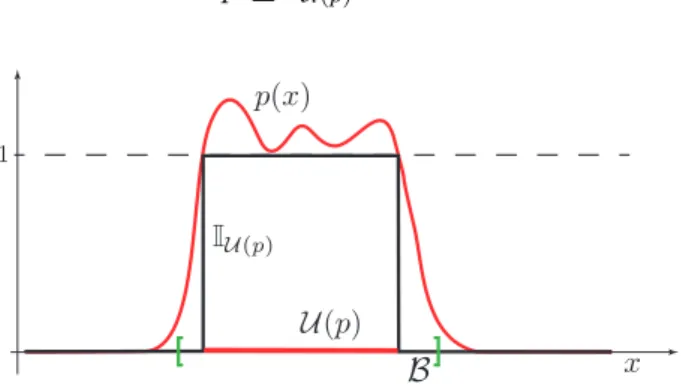
Assume now, without loss of generality, that the polynomial p used to build the PSS is non-negative on B. Then, observe that by definition of PSS (see Figure 1 for an illustration) we have
p≥IU(p) on B.
[ ]
Figure 1: Illustration of Chebychev’s inequality: the polynomial is always greater or equal than the indicator function ofp(x)≥1, hence the integral ofp overB is always an upper bound of the volume of U(p).
Hence, integrating both sides we get the following inequality Z
B
p(x)dx≥ Z
B
IU(p)(x)dx= volU(p). (7)
This inequality is indeed widely used in probability, where it goes under the name of Chebyshev’s inequality, see e.g. [2, §2.4.9]. Note that, since the polynomial p is nonneg- ative on B, then the left-hand side of inequality (7) corresponds to the L1-norm of p on B, so that the inequality simply becomes
kpk1 ≥volU(p). (8)
These derivations motivate us to the formulation of the following L1-norm minimization problem, which we choose as a surrogate of the original minimum volume outer PSS introduced in Problem 1.
Problem 2 (Minimum L1-norm outer PSS) Given a semialgebraic set K, a bound- ing set B ⊇ K, and a degree d, solve the optimization problem
wd∗ .
= inf
p∈Pd kpk1
s.t. p≥0 on B p≥1 on K.
(9)
Note that a L1-norm minimization approach was originally proposed in [23] for the nu- merical computation of the volume and of the higher order moments of a semialgebraic set. The intuition underlying the formulation of Problem 2 is similar. We now elaborate
on some of the characteristics of the minimumL1-norm outer PSS problem defined above.
First note that, for fixed d, when solving Problem 2 we are minimizing an upper-bound on the volume of the PSS. Thus, the solution is expected to be a good approximation of the set K. Second, it can be shown that, as the degree d increases, the Chebyshev bound (8) becomes increasingly tight. Indeed, the following fundamental result shows that the proposed solution converges to the minimum volume outer PSS.
Theorem 2 Given d∈N, the infimum in problem (9) is attained for a polynomial p∗d∈ Pd. Moreover, wd∗ ≥vd∗ andU(p∗d)⊇ K. Finallywd∗ ≥wd+1∗ andlimd→∞w∗d = limd→∞v∗d= volK.
Proof: Let us first extend optimization problem (9) to continuous functions:
w∗ .
= inf
f
Z
B
f(x)dx s.t. f ∈ C+(B)
f−1∈ C+(K)
(10)
whereC+(B) denotes the convex cone of non-negative continuous functions onB. Observe that since f is non-negative on B, the objective function kfk1 = R
Bf(x)dx is linear.
Problem (10) is an infinite-dimensional linear programming (LP) problem in cones of non-negative continuous functions. It has a dual LP, in infinite-dimensional dual cones of measures:
v∗ .
= sup
µ,µˆ
Z
µ(dx)
s.t. µ(dx) + ˆµ(dx) = IB(x)dx ˆ
µ∈ C+0 (B) µ∈ C+0 (K)
(11)
whereC+0 (B) is the cone of non-negative continuous linear functionals onC+(B), identified with the cone of Borel regular non-negative measures on B, according to a Riesz Repre- sentation Theorem [37, Section 21.5]. In LP (11) the right hand side in the equation is the Lebesgue measure on B. Since the mass of non-negative measures µ and ˆµ is bounded, it follows from Alaoglu’s Theorem on weak-star compactness [37, Section 15.1] that the supremum is attained in dual LP (11) and that there is no duality gap between the primal and dual LP, i.e. v∗ =w∗, see also e.g. [3, Theorem IV.7.2].
Moreover, as in the proof of [23, Theorem 3.1], it holds v∗ = volK. To see this, notice first that the constraint µ+ ˆµ=IB jointly with µ∈ C+0 (K) imply that µ≤IK and hence R µ ≤ R
IK = volK for every µ feasible in LP (11). In particular, this is true for an optimal µ∗ attaining the supremum, showing R
µ∗ =v∗ ≤ volK. Conversely, the choice µ=IK is trivially feasible for LP (11) and hence suboptimal, showing v∗ ≥R
µ= volK.
From this proof it also follows that the only optimal solution to LP (11) is the pair (µ∗,µˆ∗) = (IK,IB\K).
Now let us prove the statements of the Theorem:
• Attainment of the infimum in problem (9) follows from continuity (actually linearity) of the objective functionkpk1 =R
Bp(x)dx= 0 which is a norm (i.e. kpk1 = 0 implies
p= 0 for p∈Pd) and compactness of the set{p∈Pd : p∈ C(B), kpk1 ≤r}for any fixedr >0.
• wd∗ ≥vd∗ follows readily from (8).
• wd∗ ≥wd+1∗ follows readily from Pd⊂Pd+1.
• Finally, limd→∞wd∗ = volKis a consequence ofv∗ =w∗ = volK(proven above) and the Stone-Weierstrass Theorem [37, Section 12.3] allowing to approximate uniformly onB by polynomials any continuous function in a minimizing sequence for LP (10), i. e. limd→∞wd∗ =w∗.
.
Some remarks are at hand regarding the above result, which represents one of the main contributions of the paper.
Remark 1 (Convergence almost everywhere) Note that Theorem 2 implies that, for high enough order of approximation, the PSS obtained by minimizing the L1-norm of the polynomial defining it can be “arbitrarily close” to the semialgebraic set of interest. More precisely, as d → ∞, kp∗dk1 and, as a consequence volU(p∗d), converges to volK. Since, K ⊆ U(p∗d), the Lebesgue measure of the difference between these sets converges to zero.
In other words, one has almost everywhere convergence. From Theorems 2.5.1 and 2.5.3 in [2] the convergence is also almost uniform, up to extracting a subsequence.
Remark 2 (Trace minimization) We provide a geometric interpretation that further justifies the approximation of the minimum-volume PSS with the minimumL1-norm PSS.
To this end, we first note that the objective function in (9) reads kpk1 =
Z
B
p(x)dx= Z
B
πδT(x)P πδ(x)dx= trace
P Z
B
πδ(x)πδT(x)dx
= traceP M (12) where
M .
= Z
B
πδ(x)πδT(x)dx
is the matrix of moments of the Lebesgue measure on B in the basis πδ(x). Note that, if the basis in equation (12) is chosen such that its entries are orthonormal with respect to the (scalar product induced by the) Lebesgue measure on B, then M is the identity matrix and inequality (8) becomes
traceP ≥volU(p)
which indicates that, under the above constraints, minimizing the trace of the Gram matrix P entails minimizing the volume of U(p). It is important to remark that, in the case of quadratic polynomials, i.e. d= 2, we retrieve the classical trace heuristic used for volume minimization of ellipsoids, see e.g. [17]. Indeed, if√ B = [−1,1]n, then the basis π1(x) =
6
2 x is orthonormal with respect to the Lebesgue measure on B and kpk1 = 32traceP. Moreover, note that the constraint that p is nonnegative on B implies that the curvature of the boundary of U(p) is nonnegative, hence that U(p) is convex. Thus, U(p) is indeed an ellipsoid.
Remark 3 (Choice of B) We finally remark that, as previously noted, the assumption of the bounding set B being an hyperrectangle can be easily relaxed. Indeed, in order to develop a computationally manageable optimization in Problem 2, B can be selected as a semialgebraic set, provided that the polynomials defining the set should be such that the objective function in problem (9) is easy to compute. In particular, if
p(x) = πTd(x)p=X
α
pα[πd(x)]α
then Z
B
p(x)dx=X
α
pα Z
B
[πd(x)]αdx=X
α
pαyα and we should be able to compute easily the momentsR
B[πd(x)]αdxof the Lebesgue measure on B with respect to the basis πd(x).
4 LMI hierarchy to compute the PSS
In this section, we provide the basic details on the numerical computation of the solution of the minimumL1-norm PSS introduced in Problem 2. Note that, in problem (9), we aim at finding a polynomial p∈Pd such that i)p is positive onB, and ii) p−1 is positive on K. In order to obtain a numerically solvable problem, we enforce positivity by requiring the polynomial to be SOS, and use Putinar’s Positivstellensatz; e.g., see [36, 29, 9, 35].
More precisely, fixr ∈N, and consider the problem w2r,d∗ = min
p∈Pd
Z
B
p(x)dx (13)
s.t.
p(x) =s0,B(x) +
n
X
j=1
sj,B(x)(xj−aj)(bj −xj) s0,B ∈Σ2r
sj,B ∈Σ2(r−1), j = 1,2, . . . , n
p(x) positive on B= [a, b]
p(x)−1 = s0,K(x) +
m
X
i=1
si,K(x)gi(x) s0,K ∈Σ2r
si,K ∈Σ2(r−ri), i= 1,2, . . . , m.
p(x)−1 positive on K
where ri is the smallest integer greater than half the degree of gi for i = 1,2, . . . , m. It should be noted that the objective function of problem (13) is an easily computable linear function of the coefficients of the polynomial p. Moreover, the constraints can be recast in terms of Linear Matrix Inequalities (LMIs); see, for instance, [29]). Several Matlab toolboxes have efficient and easy to use interfaces to model problems of the form above;
e.g., see YALMIP [31].
Not only we can numerically solve problem (13), but the following result holds. This theorem is an immediate consequence of the results in [36].
Theorem 3 Let us denote by p∗2r,d a solution of problem (13). Then, the following hold i) for each d ∈ N, the value of problem (13) converges to the value of problem (9) as
r→ ∞, i.e. limr→∞w∗2r,d =w∗d, ii) for any 2r≥d, p∗2r,d ≥0 on B, iii) for any 2r≥d, p∗2r,d ≥1 on K.
We conclude that p∗2r,d can be used to compute a PSS approximation for K. For our numerical examples, we have used the YALMIP [31] interface for Matlab to model the LMI optimization problem (13) and the SDP solver SeDuMi [40] to numerically solve the problem. Since the degrees of the semialgebraic sets we compute are typically low (say less than 20), we did not attempt to use alternative polynomial bases (e.g. Chebyshev polynomials) to improve the quality and resolution of the optimization problems; see [23]
for a discussion on these numerical matters in the context of semialgebraic set volume approximation.
4.1 Computing Bounding Box B
As noted in [8, Remark 1], an outer-bounding hyper-rectangleB= [a, b] of a given semial- gebraic setKcan be found by solving relaxations of the following polynomial optimization problems
aj = arg min
x∈Rn
xj subject tox∈ K, j = 1, ..., n, bj = arg max
x∈Rn
xj subject tox∈ K, j = 1, ..., n,
which compute the minimum and maximum value of each component of the vectorxover the semialgebraic set K.
To illustrate how this can be done, let us concentrate on approximating the value of aj. First, note that the problem of computing aj is equivalent to solving the following polynomial optimization problem
aj = maxy subject to xj−y≥0 for all x∈ K.
Then, formulate the following convex optimization problem aj,2r = maxy
s.t. xj −y=s0(x) +
m
X
i=1
si(x)gi(x) s0 ∈Σ2r;
si ∈Σ2(r−ri); i= 1,2, . . . , m.
Using the same reasoning as above, it can be shown that: i) aj,2r ≤ aj for all r, and ii) limr→∞aj,2r = aj. Moreover, the problem above can be recast as an LMI optimization problem.
5 Inner approximations
The approach described in the previous sections can be readily extended to derive inner approximations of the set K, in the spirit of [10, 22, 24]. The idea is just to construct an optimal outer PSS of the complement set
K .
=B \ K ={x∈Rn :g1(x)<0 or · · · orgm(x)≤0, i= 1,2, . . . , m} ∩ B
= (K1∪ K2 ∪ · · · ∪ Km)∩ B, with Kj .
={x∈Rn :gj(x)<0}.
Note that, since the set whose indicator function we want to approximate is a union of basic semialgebraic sets, the L1 optimization problem to be solved becomes
minp∈Pd kpk1
s.t. p≥0 on B p≥1 on K1 p≥1 on K2
...
p≥1 on Km
(14)
and letp∗d attain the minimum. The corresponding optimal inner approximation is given by the polynomial sublevel set
V(p∗d) .
={x∈ B:p∗d(x)≤1}.
In this case, one can think of the polynomial 1−p∗d as a lower bound for the indicator function of the setK.
Given the fact that the optimization problem (14) provides an outer approximation of the setK, one has the following result whose proof is similar to that of Theorem 2.
Corollary 1 For all d∈N it holds V(p∗d)⊆ K. Moreover limd→∞volV(p∗d) = volK.
As before, to be able to numerically approximate the solution of problem (14), we re- place its polynomial positivity constraints by their LMI approximations as described in Section 4.
6 Numerical examples
In this section, we present several examples that illustrate the performance of the proposed approach.
6.1 Discrete-time stabilizability region
As a control-oriented illustration of the PSS approximation described in this paper, consider [22, Example 4.4] which is a degree 4 discrete-time polynomial z ∈ C 7→
x2 + 2x1z −(2x1 +x2)z3 +z4 to be stabilized by means of 2 real control parameters x1, x2. In other words, we are interested in approximating the set K of values of x1, x2 such that this polynomial has its roots with modulus less than one. An explicit basic semialgebraic description of the stabilizability region is built using the Schur stability criterion, resulting in the following basic semialgebraic set:
K ={x∈R2 : g1(x) = 1 + 2x2 ≥0, (15)
g2(x) = 2−4x1−3x2 ≥0,
g3(x) = 10−28x1−5x2−24x1x2−18x22 ≥0,
g4(x) = 1−x2−8x21−2x1x2 −x22 −8x21x2−6x1x22 ≥0}.
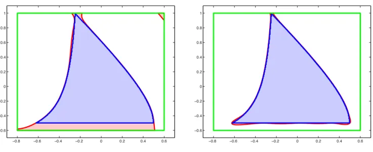
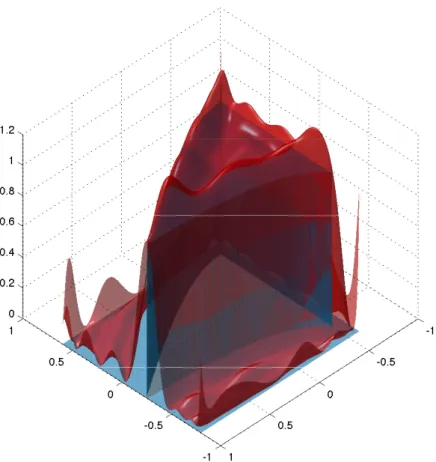
This set is nonconvex and it is included in the boxB = [−0.8,0.6]×[−0.5,1.0]. In Figure 2 we represent the PSS outer approximations of K for d = 6 and d = 12 respectively, while Figure 3 shows the graph of the degree d= 12 polynomial p∗12,12(x) constructed by solving optimization problem (13) with 2r =d.
As discussed before, we can also use the approach proposed in this paper to obtain inner approximations of K. In Figure 4, we depict the inner approximation obtained using optimization problem (14) with 2r =d= 8.
−0.8 −0.6 −0.4 −0.2 0 0.2 0.4 0.6
−0.6
−0.4
−0.2 0 0.2 0.4 0.6 0.8 1
−0.8 −0.6 −0.4 −0.2 0 0.2 0.4 0.6
−0.6
−0.4
−0.2 0 0.2 0.4 0.6 0.8 1
Figure 2: Degree 6 and degree 20 outer PSS approximation (red) of stabilizability region K (inner surface in light blue). The green box corresponds to the bounding set B.
Figure 3: Degree 20 polynomial approximation (upper surface in red) of the indicator function (lower surface in blue) of the nonconvex planar stabilizability regionK.
6.2 PID stabilizability region
We now turn our attention to an example related to fixed order controller design. Consider [6, Example 2.2], in which the authors examine the problem of stabilizing the plant P(s) = N(s)D(s) where
N(s) = s3−2s2 −s−1;
D(s) = s6+ 2s5+ 32s4+ 26s3+ 65s2−8s+ 1.
by means of a PID controller of the formKPID(s) = kP+ksI +kDs. In particular, they are interested in finding the set of stabilizing PID gains, that is the set of gains for which the closed-loop characteristic polynomialsD(s) + (kI+kPs+kDs2)N(s) is Hurwitz. For this special class of controllers, the authors provide a method based on the so-called signature of a set of properly constructed polynomials to determine the set of all PID gains that stabilize the plant. One should note that this procedure is not easily generalizable to more general classes of fixed order controllers.
In our setup, we are interested in approximating the set
K={x∈R3 :sD(s)+(kI+kPs+kDs2)N(s) is Hurwitz, kI = 25(x1−1), kP = 10(x2−1.5), kD = 10(x3−1)}
with bounding boxB = [−1,1]3. As one can see in Figure 5, the approached proposed in
−0.8 −0.6 −0.4 −0.2 0 0.2 0.4 0.6
−0.6
−0.4
−0.2 0 0.2 0.4 0.6 0.8 1
Figure 4: Left: degree 8 inner PSS approximation (red) of stabilizability region K(inner surface in light blue). Right: degree 8 polynomial approximation (upper surface in red) of the indicator function (lower surface in blue ofK.
this paper provides a very good approximation of the set of stabilizing gains, even for a PSS of relatively low order (d= 14).
7 Reconstructing/approximating Sets from a finite number of samples
A particularly interesting case is when the semialgebraic set K is discrete, that is, it consists of the union ofN points
K=
N
[
i=1
{x(i)} ⊂Rn.
This situation arises for instance when the objective is to try to approximate a given set (possibly non-semialgebraic) from a given number of points in its interior. An example of this is the reconstruction of reachable sets by using randomly generated trajectories.
This setup is discussed in [14, 13, 25].
From a computation viewpoint, an important feature is that, in the case of a discrete set, the inclusion constraint K ⊆ U(p) is equivalent to a finite number of inequalities
p(x(i))≥1, i= 1, . . . , N
which are linear in the coefficients of p. This fact allows to deal with problems with rather largeN. Moreover, in this latter case, where the number of pointsN is large while
Figure 5: Left: set of stabilizing PID gains. Right: its degree 14 optimal outer PSS approximation.
the dimension n is relatively small, the constraint that pis nonnegative on B can also be (approximately) handled by linear inequalities
p(z(j))≥0, j = 1, . . . , M
enforced at a dense grid of pointsz(j) ∈ B, forM sufficiently large. Hence, in this case one can construct a pure linear programming (LP) approach. Note that, even if this approach does not guarantee thatpis nonnegative everywhere on B, it still ensures that K ⊆ U(p), which is what matters primarily in our approach.
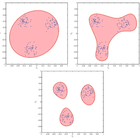
To illustrate the performance of the proposed method, we first consider N = 100 points in the box B = [−1, 1]2. The points are generated mapping Gaussian points with vari- ance 0.1I and mean value chosen with equal probability between [0.4, 0.3]T, [−03, −0.5]T, [−0.5, 0.4]T. On Figure 6 we represent the solutionspof degrees 2, 5, and 9 of minimiza- tion problem (9). A few comments about the obtained solution are at hand. First, we see that the solution for d = 2 corresponds to the L¨owner-John ellipsoid, see e.g. [4, §4.9].
Second, it can be observed that, as the degree of p increases, the set U(p) becomes dis- connected, so as to better capture the different regions where the points are concentrated.
We note that, in the case of discrete points, it is not advisable to select high values of d, since indeed, in the limit, the optimal polynomial would correspond to a function with spikes corresponding to the location of the considered points. Finally, we remark that the possible side effects near the border ofB on the right hand side figure can be removed by enlarging the bounding set B.
As a second illustrative example, we considerN = 10 points inB= [−1,1]3. The solutions p of degrees 4, 6, 9, and 14 of minimization problem (9) is depicted in Figure 7. Here
x1 x2
−1 −0.8 −0.6 −0.4 −0.2 0 0.2 0.4 0.6 0.8 1
−1
−0.8
−0.6
−0.4
−0.2 0 0.2 0.4 0.6 0.8 1
x1 x2
−1 −0.8 −0.6 −0.4 −0.2 0 0.2 0.4 0.6 0.8 1
−1
−0.8
−0.6
−0.4
−0.2 0 0.2 0.4 0.6 0.8 1
x 1 x2
−1 −0.8 −0.6 −0.4 −0.2 0 0.2 0.4 0.6 0.8 1
−1
−0.8
−0.6
−0.4
−0.2 0 0.2 0.4 0.6 0.8 1
Figure 6: MinimumL1-norm PSS at 100 points (blue), for degree 2 (left), 5 (center), and 9 (right).
too we observe that increasing the degree ofp allows to capture point clusters in distinct connected components.
8 Uniform sampling over semialgebraic sets
In this section, we consider a problem that can be seen as the “dual” of the one considered in the previous section; that is, instead of trying to reconstruct/approximate the indicator function of an unknown set from points belonging to its interior, we aim at developing systematic procedures for generating uniformly distributed samples in a given semialge- braic set. This is an important problem since many system specifications lead to sets with a (complex) closed-form description, and being able to draw samples from these type of sets provides the means for the design of systems with a complex set of specifications.
In particular, the algorithm presented in this section can be used to generate uniform samples in the solution set of LMIs.
As before, we assume that the set of interest is a compact basic semialgebraic set defined as in (1), and that there exists a bounding hyper-rectangle B = [a, b] of the form (6).
Then, the problem we discuss in this section is the following.
Figure 7: Including the same 10 space points (blue) in PSS of degree 4 (left) and 10 (right).
Problem 3 (Uniform Sample Generation over K) Given a semialgebraic set K de- fined in (1) of nonzero volume, generate N independent identically distributed (i.i.d.) random samples x(1), . . . , x(N) uniformly distributed in K.
Let us start by describing the approach proposed to solve this problem. First, we define the uniform density over the set Kas follows
UK .
= IK
volK (16)
where IK is the indicator function of the set K defined in (3). Then, the idea at the basis of the proposed method is to use a PSS approximation of the setKor, equivalently, a polynomial over approximation of the indicator function IK, obtained employing the framework introduced in Sections 2 and 3.
To this end, given a degreed∈N, consider the optimization problem (9) and let p∗d be a polynomial that achieves the optimum. If one examines the proof of Theorem 2, one can see that this polynomial has the following properties
i) p∗d ≥IK onB
ii) As d→ ∞, p∗d→IK both in L1 and almost uniformly on B.
Hence, p∗d can arbitrarily approximate (from above) the indicator function of the set K., and therefore it represents a so-called “dominating density” of the uniform densityUK on B. More formally, there exists a value β > 0 such that βp∗d(x) ≥ UK(x) for all x ∈ B.
Hence, the rejection method from a dominating density, discussed for instance in [41, Section 14.3.1], can be applied leading to the following random sampling procedure.
A graphical interpretation of the algorithm is provided in Figure 8, for the case of a simple one-dimensional set
K=
x∈R : (x−1)2−0.5≥0, x−3≤0 .
Algorithm 1Uniform Sample Generation in Semialgebraic Set K Given d∈N, let p∗d be a solution of
minp∈Pd
Z
B
p(x)dx s.t. p≥1 on K
p≥0 on B.
(17)
1. Generate a random sample ξ with density proportional to p∗d overB.
2. If ξ 6∈ Kgo to step 1.
3. Generate a sample u uniform on [0, 1].
4. If u p∗d(ξ)≤1 return x=ξ, else go to step 1.
First, problem (9) is solved (for d= 8 and B= [1.5, 4]), yielding the optimal solution
p∗d(x) = 0.069473x8−2.0515x7+23.434x6−139.5x5+477.92x4−961.88x3+1090.8x2−606.07x+107.28.
As it can be seen in Figure 8, p∗d is “dominating” the indicator function IK on B. Then, uniform random samples are drawn in the hypograph of p∗d. This is done by generating uniform samples ξ distributed according to a probability density function (pdf) propor- tional to p∗d (step 2), and then selecting its vertical coordinate uniformly in the interval [0, ξ] (step 3). Finally, if this sample falls below the indicator function IK (blue dots) it is accepted, otherwise it is rejected (red dots) and the process starts again.
1.5 2 2.5 3 3.5 4
−0.5 0 0.5 1 1.5
Figure 8: Illustration of the behavior of Algorithm 1 in the one-dimensional case. Blue dots are accepted samples, red dots are rejected samples.
It is intuitive that this algorithm should outperform classical rejection from the bounding set B, since more importance is given to the samples inside K through the function p∗d.
To formally analyze the performance of Algorithm 1, we define the acceptance rate (see e.g. [16]) as the reciprocal of the expected number of samples that have to be drawn fromp∗d in order to find one “good” sample, that is a sample uniformly distributed in K.
Then, the following result, which is the main theoretical result of this section, provides the acceptance rate of the proposed algorithm.
Theorem 4 Algorithm 1 returns a sample uniformly distributed in K. Moreover, the acceptance rate of the algorithm is given by
γd= volK w∗d , where w∗d .
=R
Bp∗d(x)dx is the optimal solution of problem (9).
Proof: To prove the statement, we first note that polynomial p∗d defines a density f .
= p∗d
w∗d (18)
overB. Moreover, by construction, we havep∗d ≥IK onB, and hence p∗d
w∗dvolK ≥ IK
w∗dvolK (19)
f
volK ≥ UKf
w∗d ≥γdUK
onB. Then, it can be immediately seen that Algorithm 1 is a restatement of the classical Von Neumann rejection algorithm, see e.g. [41, Algorithm 14.2], whose acceptance rate is given by the value of γd such that (19) holds, see for instance [15].
It follows that the efficiency of the random sample generation increases as d increases, and becomes optimal as d goes to infinity, as reported in the next corollary.
Corollary 2 In Algorithm 1, the acceptance rate tends to one when increasing the degree of the polynomial approximation, i.e.
d→∞lim γd= 1.
Therefore, a trade-off exists between the complexity of computing a good approximation (d large) on the one hand, and having to wait a long time to get a “good” sample (γ large), on the other hand. Note, however, that the first step can be computed off-line for a given setK, and then the corresponding polynomial p∗d can be used for efficient on-line sample generation. Finally, we highlight that, in order to apply Algorithm 1 in an efficient way (step 2), a computationally efficient scheme for generating random samples according to a polynomial density is required. This is discussed next.
8.1 Sample generation from a polynomial density
To generate a random sample according to the multivariate polynomial densityf defined in (18), one can use the so-called conditional density method described in [15]. This is a recursive method in which the individual entries of the multivariate samples are generated according to their conditional probability density. We now elaborate on this.
We should note that the approach developed in this paper only provides the density up to a multiplying constant. However, to simplify the exposition to follow, we proceed as if the polynomial given is indeed a probability density function.
Assume that the bounding set is a hyperrectangle B = [a, b] of the form (6) and that we have a polynomial densityp. We start by computing the marginal density
p1 :x1 7→
Z b2
a2
· · · Z bn
an
p(x1, x2, . . . , xn) dx2· · ·dxn
and, for each i= 2, . . . , nand given ¯x1, . . .x¯i−1, compute conditional marginal densities pi :xi 7→
Z bi+1
ai+1
· · · Z bn
an
p(¯x1, . . . ,x¯i−1, xi, xi+1, . . . , xn)dxi+1· · ·dxn
and respective (polynomial) cumulative distributions Fi satisfying dFi
dxi =pi.
The sampling procedure then starts by computing a sample ¯x1 according to F1 and, iteratively, computing samples ¯xi given ¯x1, . . .x¯i−1 according to the distribution Fi. The exact description of this procedure is described in Algorithm 2. One should note that, given the densityp, a closed form is available for all marginal and conditional densities. In other words, none of the integrations mentioned above needs to be computed numerically.
8.2 Numerical example: sampling in a nonconvex semialgebraic set
To demonstrate the behavior of Algorithms 1 and 2, we revisit Example 6.1, and generate uniform samples in the semialgebraic set K defined in (15). As already shown in Figure 3, the indicator functionIK is well approximated from above by the optimal PSSp∗d,d for d= 20. The results of Algorithm 1 are reported in Figure 9. The red points represent the points which have been discarded. To this regard, it is important to notice that also some point falling inside K has been rejected. This is fundamental to guarantee uniformity of the discarded points.
9 Concluding Remarks
In this paper we have introduced the concept of polynomial superlevel sets (PSS) as a tool to construct “simple” approximations of complex semialgebraic sets. Algorithms are
Algorithm 2Generation from a polynomial density
Returns a sample inB[a,b] with density proportional to the polynomial p: x1, . . . , xn 7→
nα
X
j=1
pj
n
Y
`=1
xα`j,` (20)
1. Let i= 1
2. Compute the univariate polynomial F : xi 7→
nα
X
j=1
γi,j(¯x1, . . . ,x¯i−1)xαij,`+1 (21)
where
γi,j(¯x1, . . . ,x¯i−1) = 1 aj,i+ 1pj
i−1
Y
`=1
¯ xα`j,`
! n Y
`=j+1
1 αj,`+ 1
bα`j,`+1−aα`j,`+1
! (22)
3. Generate a random variable w uniform on [F(ai), F(bi)]
4. Compute the unique root ξi in [ai, bi] of the polynomial xi 7→ F(xi)−w 5. Let ¯xi =ξi
6. If i < n let i=i+ 1 and go to (2) 7. Return ¯x
provided for computing these approximations. Moreover, it is shown how this concept can be used to solve two important problems: i) reconstruction/approximation of sets from samples and ii) generation of uniform samples in basic semialgebraic sets. Examples of the application of these ideas to problems in control engineering are also described. Note that the methods provided in this paper can be used to obtain probabilistic approximations of difficult sets, in the spirit of what is discussed in [14]. Also, in [13] the application of minimum size PSS to the approximation of the one-step reachable set of a nonlinear discrete-time function is presented, with an extension to nonlinear set filtering. Finally, we note that similar techniques can also be used to approximate transcendental (i.e.
non-semi-algebraic) sets arising in systems control, e.g. regions of attraction, maximum positively invariant sets, and controllability regions.
References
[1] T. Alamo, J.M. Bravo, and E.F. Camacho. Guaranteed state estimation by zono- topes. Automatica, 41(6):1035–1043, 2005.
Figure 9: Uniform random samples generated according to Algorithms 1 and 2. The light blue area is the set K defined in (15), the pink area is the PSS U(p∗d). The red dots are the discarded samples. The remaining samples (blue) are uniformly distributed insideK.
[2] R.B. Ash and C.A. Dol´eans-Dade. Probability and measure theory, 2nd edition. Aca- demic Press, San Diego, CA, 2000.
[3] A. Barvinok. A course in convexity. American Mathematical Society, Providence, USA, 2002.
[4] A. Ben-Tal and A. Nemirovski. Lectures on modern convex optimization. SIAM, Philadelphia, PA, 2001.
[5] D. Bertsimas, X. Vinh Doan, and J.B. Lasserre. Optimal data fitting: a moment ap- proach. Research report, Sloan School of Management, MIT, Boston, MA, February 2007.
[6] S.P. Bhattacharyya, Datta A, and L.H. Keel. Linear Control Theory: Structure, Robustness, and Optimization. Springer-Verlag, Boca Raton, 2009.
[7] V. Cerone, D. Piga, and D. Regruto. Polytopic outer approximations of semialgebraic sets. In Proc. of the IEEE Conference on Decision and Control, 2012.
[8] V. Cerone, D. Piga, and D. Regruto. Polytopic outer approximations of semialgebraic sets. In Proc. of the IEEE Conference on Decision and Control, pages 7793–7798, 2012.
[9] G. Chesi, A. Garulli, A. Tesi, and A. Vicino. Solving quadratic distance problems: An LMI-based approach. IEEE Transactions on Automatic Control, 48:200–212, 2003.
[10] F. Dabbene, P. Gay, and B.T. Polyak. Recursive algorithms for inner ellipsoidal approximation of convex polytopes. Automatica, 39(10):1773–1781, 2003.