HAL Id: hal-01403915
https://hal.archives-ouvertes.fr/hal-01403915
Submitted on 28 Nov 2016
HAL
is a multi-disciplinary open access archive for the deposit and dissemination of sci- entific research documents, whether they are pub- lished or not. The documents may come from teaching and research institutions in France or
L’archive ouverte pluridisciplinaire
HAL, estdestinée au dépôt et à la diffusion de documents scientifiques de niveau recherche, publiés ou non, émanant des établissements d’enseignement et de recherche français ou étrangers, des laboratoires
A non-staggered coupling of finite element and lattice Boltzmann methods via an immersed boundary scheme
for fluid-structure interaction
Zhe Li, Julien Favier
To cite this version:
Zhe Li, Julien Favier. A non-staggered coupling of finite element and lattice Boltzmann methods via
an immersed boundary scheme for fluid-structure interaction. Computers and Fluids, Elsevier, 2017,
143, pp.90 - 102. �10.1016/j.compfluid.2016.11.008�. �hal-01403915�
A non-staggered coupling of finite element and lattice Boltzmann methods via an immersed boundary scheme
for fluid-structure interaction
Zhe Lia,∗, Julien Favierb
aLHEEA laboratory, ´Ecole Centrale de Nantes, UMR CNRS, Nantes, France
bAix-Marseille Universit´e, CNRS, Centrale Marseille, M2P2 UMR 7340, Marseille, France
Abstract
The paper presents a numerical framework for the coupling of finite element and lattice Boltzmann methods for transient problems involving fluid-structure interaction. The solid structure is discretized with the finite element method and integrated in time with the explicit Newmark scheme. The lattice Boltzmann method is used for the simulation of single-component weakly-compressible fluid flows. The two numerical methods are coupled via a direct-forcing immersed boundary method in a non-staggered way. Without subiteration within each time-step, the proposed method can ensure the synchronization of the time integrations, and thus the strong coupling of both subdomains by resolving a linear system of coupling equations at each time-step. Hence the energy transfer at the fluid-solid interface is correct, i.e. neither energy dissipation nor energy injection will occur at the interface, which can retain the numerical stability.
A well-known fluid-structure interaction test case is adopted to validate the proposed coupling method. It is shown that the stability of the used numerical schemes can be preserved and a good agreement is found with the reference results.
Keywords: finite element method, lattice Boltzmann method, immersed boundary method, fluid-structure interaction, interface-energy-conserving
∗Corresponding author
Email address: Zhe.Li@ec-nantes.fr(Zhe Li)
1. Introduction
Fluid-Structure Interaction (FSI) refers to interactions between two kinds of media, namely the fluid flow and the solid structure. Well-known examples include wind-induced oscillations of tall buildings, collapse of bridges caused by wind gusts, flow-induced vibrations of airfoils, and dynamics of blood flow through valves in veins etc. Thus, the robustness and accuracy of the numerical methods used for their simulations are of primary importance. Due to the different material and dynamical properties of fluid and solid media, one feature of FSI simulation is that the fluid and solid subdomains are generally modelled using different numerical methods, e.g. Eulerian fashion for fluid and Lagrangian fashion for solid, and different discretizations, both in space and time. In this paper, we propose a numerical framework to simulate two-way FSI problems by means of the coupling of Finite Element (FE) method for deformable solid structure and Lattice Boltzmann (LB) method for weakly-compressible fluid flow.
To simulate the solid structure, we adopt the FE method [1, 18], which is widely used in solving solid dynamics. Based on the total Lagrangian formula- tion [1], the adopted FE solver can be used to handle geometrical nonlinearities, such as moderate deformation-large rotation cases. For time integration, we choose to use the Newmark scheme [28] which enjoys great popularity due to its “single-step, single-solve” feature in linear as well as in nonlinear dynamic analysis. Besides, the Newmark time integrator also features controllable energy dissipation with two coefficients of the scheme [20]. More details of the chosen Newmark scheme will be discussed subsequently.
The fluid subdomain is simulated with the LB method, which is gaining much attention over the past decade. As an alternative to conventional numer- ical solvers based on the resolution of Navier-Stokes (NS) equations, the LB method consists in solving the discrete Boltzmann equation with collision and streaming processes, which can be proven to fully recover the macroscopic NS equations through the Chapman-Enskog analysis [3]. Recently, Shan et al. [34]
have shown that the LB method can be systematically derived from the kinetic theory for hydrodynamics. In the present work, we apply the single-component isothermal LB model for the simulation of a weakly compressible laminar fluid flow interacted with a deformable solid structure via an Immersed Boundary (IB) method.
Initially proposed by Peskin [29] for simulating blood flows in the hearts, IB method is particularly useful for introducing moving solid objects in the fluid domain modelled with a fixed Eulerian mesh, which is the case for LB method.
Since its appearance, IB method has many variants [27]. Recently, several IB- LB coupled schemes have been presented for simulating FSI problems: Wu and Shu [38, 39] proposed an implicit velocity correction-based IB-LB method for one-way (stationary solid boundary) FSI simulations; Favier et al. [12]
proposed an IB-LB coupling scheme based on a prediction-correction substage within each time-step, which was applied to simulate the fluid interaction with moving and slender flexible objects; de Rosis [7] proposed an iterative strong IB-LB coupling method for simulating two-way FSI problems in the presence of slender deformable solid. In the present paper, we adopt the direct-forcing IB method proposed in [22], which can enforce the no-slip condition at the immersed boundaries by using an appropriate local width for each Lagrangian point.
In the previous publications [4, 19, 21], different FE-LB coupling strategies have been proposed for the simulation of FSI problems in the presence of de- formable solid structure. However, all of them can be classified as staggered coupling procedures [13], in which there always exists a lag between the time integrations of fluid and solid subdomains. For example, in [4], the force vec- tor for the FE solver needed to be guessed with a force predictor, because the fluid-structure coupling determines the effective force. In [21], one takes the interface forcefn at the moment tn to compute the fluid velocityun+1 at the next momenttn+1, which actually depends onfn+1; in order to reduce the time lag, structural predictors [31] have been used in [19, 21] to obtain a numerically stable simulation. This time-lag may sometimes degrade the stability or con-
vergence order of the numerical schemes. In spite of the staggered feature, the advantage of these coupling strategies is that one does not need to significantly modify the existing codes or softwares for the FSI implementation.
The main objective of the present paper is to present a synchronous or non- staggered FE-LB coupling framework without subiteration within each time- step via a direct-forcing IB method. The non-staggered and subiteration-free features make the proposed coupling method robust and efficient, respectively.
Indeed, coupling of heterogeneous numerical methods may be of great impor- tance in terms of preserving numerical stability for FSI computations, especially when a partitioned coupling algorithm is adopted. Unlike monolithic coupling procedure, which treats computationally the fluid and solid subdomains as an entity, the partitioned procedure allows us to carry out separately the time inte- gration of each subdomain [13]. This is particularly convenient when one prefers to solve the fluid and solid equations using different numerical methods or ex- isting softwares, which are already designed and optimized for each individual subdomain [11]. However, partitioned coupling algorithm often suffers numer- ical instabilities, if no special synchronization techniques, such as subiterative methods [10] or structural predictors [31], are applied. With this kind of cou- pling procedure, e.g. the Conventional Serial Staggered (CSS) method [13, 31], the FSI computation may diverge rapidly, even though the individual schemes used in the fluid and solid subdomains are both numerically stable. This is usually due to the time lag between the time integrations of the fluid and solid subdomains [23, 24, 26, 31].
From the energy point of view [5, 6, 8, 15], this CSS coupling procedure algorithmically injects or dissipates energy at the fluid-solid interface. When too much algorithmic interface energy is injected to the system, the coupling simulation will be interrupted due to the numerical instability. In the context of FE-LB coupling method, Kollmannsberger et al. [19] have proposed a nu- merical framework for FSI simulations, in which they applied and evaluated the basic and improved CSS [13] coupling algorithms with the interface-energy- conservation criteria. They showed that with the first order structural predictor
one can have a numerically stable simulation for the specific test case. However, as they showed in the comparison, using an elaborate structural predictor in a staggered coupling procedure can only reduce the increasing artificial interface energy, i.e. it cannot ensure exactly a zero interface energy. Consequently, the numerical stability of the FSI simulation will highly depend on the investigated problem.
In summary, the most important feature of the proposed FE-LB coupling method is that it can rigorously ensure the zero-interface-energy condition dur- ing the whole period of numerical simulation, in such a way that the numerical stability can be preserved for the FSI computations. The key point of this method is to construct a linear system of coupling equations at each time-step.
By resolving the equations with the dual Schur formulation [14], one can update the interface velocity and force to the next time-step. Since the interface veloc- ity and force are resolved simultaneously, the interface status update is implicit.
But it is worth noting that this implicit updating procedure is based on solv- ing directly a linear system of equations, rather than based on a subiterative coupling procedure [7, 36].
The rest of the paper is organized as follows: Section 2 gives the mathe- matical formulations of the used numerical methods (FE, LB and IB methods);
Section 3 starts with a brief presentation of the time lag issue for staggered methods in the framework of FE-LB coupling with Newmark time integrator, and then presents the proposed non-staggered coupling method; Section 4 shows the numerical results of the validation test cases; finally, the conclusions and dis- cussions are drawn in Section 5.
2. Mathematical formulation and numerical methods
2.1. Finite element method for solid structure
2.1.1. Semi-discrete equations obtained through total Lagrangian formulation As presented in [1], the weak total Lagrangian formulation for solid can be obtained by integrating the momentum equation multiplied by a virtual
displacement field over the initial configuration:
Z
Ω0s
δus·
ρ0s∂2us
∂t2 −∇0·P−ρ0sb
dΩ0s= 0 (1)
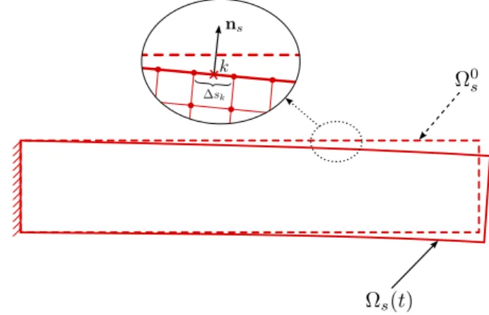
where Ω0s(X) denotes the solid initial configuration, as shown in Figure 1, with X being the time-independent Lagrangian or material coordinate. In addition, δus(X) denotes the virtual displacement field,ρ0s(X) the initial solid density, us(X, t) the solid displacement field defined asus(X, t) =x−Xwherex(X, t) denotes the Eulerian or spatial coordinate of the material pointXin the current solid configuration Ωs(t). P(X, t) is the nominal stress tensor and ∇0·is the divergence operator with respect to the material coordinateX. Finally,b(X, t) is the body force vector per unit mass such as the gravity.
Figure 1: Initial and current solid configurations.
Eq. (1) is also referred to as the virtual work principle that can give us the semi-discrete solid equations in matrix form [1]:
Msas=fext−fint (2) whereas denotes the acceleration field defined as:
as= dvs
dt vs= dus
dt
(3)
with the displacement fieldus = [u1s, . . . ,uIs, . . . ,uNs ]⊤, the velocity fieldvs = [v1s, . . . ,vIs, . . . ,vsN]⊤ and the acceleration field as = [a1s, . . . ,aIs, . . . ,aNs ]⊤, in whichuIs= [uI,xs (t), uI,ys (t)],vIs= [vsI,x(t), vI,ys (t)] andaIs= [aI,xs (t), aI,ys (t)] are theIth node’s displacement, velocity and acceleration inx- andy-directions in 2D cases.
Additionally,Ms,fintandfextare the mass matrix, the internal and external nodal forces, respectively, which are given as:
MIJs =I Z
Ω0s
ρ0sNINJ dΩ0s fintI ⊤
= Z
Ω0s
BI0⊤ PdΩ0s fextI =
Z
Ω0s
NIρ0sb0 dΩ0s+ Z
Γ0s
NIλ0dΩ0s
(4)
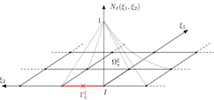
whereIis the identity matrix,NI(X) and NJ(X) are the shape functions for the used 4-nodes quadrangle element at the Ith and Jth nodes, as shown in Figure 2.
The constant matrixBI0 is given as:
BI0⊤
= ∂NI
∂X ,∂NI
∂Y
(5) whereXandY are the Lagrangian coordinates inx- andy-directions. Moreover, the nominal stress tensor P is calculated by P = S·F⊤ with S being the second Piola-Kirchhoff (PK2) stress andF=∂x/∂X denoting the deformation gradient. In the present work, we consider an elastic solid structure, hence the PK2 stressSis linearly related to the Green-Lagrange strain Eby means of a constant fourth-order tensor C, i.e. S = C : E where E = 1/2(F⊤·F−I), which is referred to as the Saint Venant-Kirchhoff material model.
In the present paper, no external body force is considered for the structure, henceb0=0. In addition,λ0 denotes the external surficial force acted on the initial configuration Ω0s.
Figure 2: Shape function for the 4-nodes quadrangle element at theIth node in the parent configuration Ωξs.
2.1.2. Time integration with Newmark scheme
To integrate in time this semi-discrete system of equations (2), we choose to apply the Newmark time integrator [28]:
un+1s =uns + ∆tvns+∆t2 2
(1−2β)ans+ 2βan+1s vsn+1=vns + ∆t
(1−γ)ans +γan+1s (6)
where the superscripts n and n+ 1 indicate the time instants tn and tn+1 for the displacement us, velocityvs and the acceleration as. In addition, ∆t denotes the constant time-step, which is the same for both the solid and fluid subdomains. Finally,β andγ are the two coefficients of the Newmark scheme.
In the present work, we chooseβ= 0 andγ= 0.5 for the solid simulations, with which the Newmark time integrator is essentially an explicit central difference scheme possessing second-order accuracy in time and conditional stability. The time-step ∆tshould be smaller than the critical time-step ∆tcritdetermined by [1]:
∆t <∆tcrit= min
e
le
ce
(7) whereledenotes the characteristic length of theethelement andceis the current wave speed in theeth element. Because the simulations are carried out with a constant time-step ∆t, one has to preset a ∆tunder the stability condition (7).
It is here noteworthy that although the condition (7) is valid only for linear
cases, it can provide a useful guide for choosing the time-step in nonlinear cases [1]. In this work, we estimate ∆tcrit by setting le = ∆X and ce = p
Es/ρ0s where ∆X denotes the initial uniform spacing of the solid mesh andEs is the Young’s modulus of the elastic solid material.
2.1.3. Calculation of external nodal force vector with a geometric operator In the present work, the FSI happens only at the fluid-solid interface ΓI. For the FE solver, the velocity boundary condition is tackled with the elimination method, and the time-varying force boundary condition is imposed by using a geometric operatorLp that relates the external nodal forcefext with the flow- induced forceΛas fext=−LpΛ:
fext1 fext2 ... fextNs
| {z }
fext
=−
L1,1p L1,2p . . . L1,Np k L2,1p L2,2p . . . L2,Np k
... ... . .. ... LNps,1 LNps,2 . . . LNps,Nk
| {z }
Lp
λ1
λ2
... λNk
| {z }
Λ
(8)
where fextI = [fextI,x, fextI,y]⊤ is the external nodal force for the node I ∈ [1, Ns] with Ns being the total number of the solid nodes. λk = [λxk, λyk]⊤ denotes the force per unit length in 2D cases, which is exerted on thekth (k∈[1, Nk]) fluid-solid interface element, as shown in Figure 1, andNk is the total number of the interface elements.
It is worth noting that this geometric operatorLpis time-varying and entirely depends on the current solid geometry. As mentioned previously, we choose to use the explicit Newmark scheme withβ = 0 andγ = 0.5, which allows us to explicitly calculate the new displacement field un+1s =uns+ ∆tvn+ 0.5∆t2ans so that we can explicitly update the solid geometry with this newly obtained displacement fieldun+1s . By doing so, we avoid the iterative procedure usually required for the implicit Newmark schemes to handle such geometrical nonlin- earity.
To construct the geometric operatorLp, we follow the way proposed by the author in the previous work [24] for the coupling of SPH and FE methods. As
one can observe in Equation (8), if one imposes a force boundary condition λxk =−1 andλyk = 0, λxm = 0 and λym = 0 withm ∈[1, Nk] and m6=k, then the (2k−1)thcolumn ofLpis just the external nodal forcefextunder such force boundary condition. Similarly, the 2kth column ofLp is the external forcefext with the force conditionλxk = 0 and λyk =−1,λxm= 0 andλym= 0. Moreover, the formulae for calculatingfextis given as follows:
fextI = Z
Γ0I
NIλ0 dΓ0I = Z
ΓI
NIλdΓI (9)
where ΓI(t) is the current interface that is constituted ofNk interface element, i.e. ΓI =P
kΓk. λ(x, t) denotes the external force acted on the current solid configuration. Here we assume that the force is piece-wise constant at the interface and is applied on the geometric center of each element Γk. Following the method presented previously, only one interface element is charged at each time, hencefextcan be calculated as:
fextI =λk
Z
Γk
NI dΓk=λk
Z
Γξk
NIJξ dΓξk=
λxk λyk
∆sk
∆sξk (10) where Γξk represents the element k in the parent domain as shown in Figure 2, and Jξ = ∆sk/∆sξk is the Jacobian of the mapping from the current to the parent configurations, with ∆sk and ∆sξk being the element length (2D) in the current and parent configurations, respectively.
2.2. Lattice Boltzmann method for single-component fluid flow
In the lattice Boltzmann method the fluid state is updated by resolving the discrete Boltzmann equation:
fi(x+ci∆t, t+ ∆t) =fi(x, t)−∆t
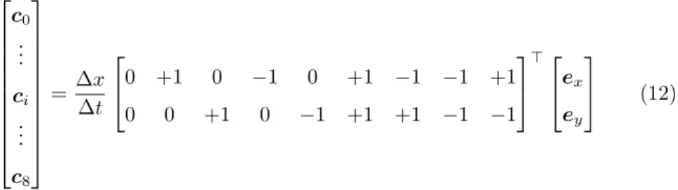
τ [fi(x, t)−fieq(x, t)] + ∆tGi(x, t) (11) wherefi(x, t) denotes the distribution function at the sitexand the timet, in theith direction of the used D2Q9 [32] lattice for 2D cases, as shown in Figure 3, andci is theith discrete velocity vector. The set of discrete velocity vectors
of D2Q9 lattice can be obtained in the following way:
c0
... ci
... c8
= ∆x
∆t
0 +1 0 −1 0 +1 −1 −1 +1
0 0 +1 0 −1 +1 +1 −1 −1
⊤
ex
ey
(12)
where ∆xdenotes the uniform spacing of the lattice, ∆t is the constant time- step, andexandey are two unit vectors inx- andy-directions.
1 2
3
4
5 6
8 7
0 x
y
Figure 3: The D2Q9 lattice used in the present work for 2D LB simulations.
In Equation (11), the single-relaxation-time Bhatnagar-Gross-Krook (BGK) collision model is adopted and τ denotes the relaxation time. Here, fieq(x, t) is referred to as the discrete equilibrium distribution function, which can be obtained by Hermite series expansion of the Maxwell-Boltzmann equilibrium distribution [34]:
fieq=ρfωi
"
1 + ci·vf
c2s,f +(ci·vf)2
2c4s,f −vf·vf
2c2s,f
#
(13) where ρf(x, t) andvf(x, t) denote the macroscopic fluid density and velocity, cs,f =p
1/3∆x/∆t the speed of sound, andωi the weight coefficients equaling ω0 = 4/9, ω1−4 = 1/9 andω5−8 = 1/36 for D2Q9 lattice. In such isothermal single-component LB model the fluid pressure is calculate aspf=c2s,fρf and the kinematic viscosityν is related to the relaxation timeτ byν=c2s,f(τ−0.5∆t).
Additionally, we adopt the scheme proposed by Guo et al. [16] in order to take into account the body-force effects in the fluid domain. In Equation (11),
the body-force-related termGi(x, t) is given as [16]:
Gi =
1−∆t 2τ
ωi
"
ci−vf
c2s,f +(ci·vf) c4s,f ci
#
·F (14) whereF(x, t) denotes the body force per unit volume acted on fluid at the site xand the timet.
Finally, once one calculates all the distribution functions fi(x, t+ ∆t) by means of Equation (11), we can update the macroscopic fluid status by the definition [16]:
ρf =X
i
fi
ρfvf =X
i
cifi+∆t 2 F
(15)
Note that this definition of the macroscopic fluid velocity should be used at each time instant in order to make the LB scheme fully recover the Navier-Stokes equations.
In the present work, no gravity effect is considered in the fluid subdomain, hence the body forceF in Equation (15) is just the force related to the immersed boundary method, which is used to relate the fluid and solid subdomains for FSI simulations.
2.3. Immersed boundary method
In this paper, we apply the IB method proposed by the authors in the previous work [22], in which the IB method was used to impose moving solid boundary conditions in the fluid flow. This IB method is based on the interpo- lated definition of the macroscopic fluid velocity (15) from the Eulerian (fluid) nodes to the Lagrangian (solid) points:
I[ρf]kvf,k =I
"
X
i
cifi
#
k
+∆t
2 Fk (16)
wherevf,k andFk denote the fluid velocity and the IB-related force at the kth solid element, respectively. I[•]k represents the interpolation operator defined
as:
φ(xk, t) =I[φ(x, t)]k= Z
φ(x, t)δ(x−xk) dx
≃ X
j∈Dk
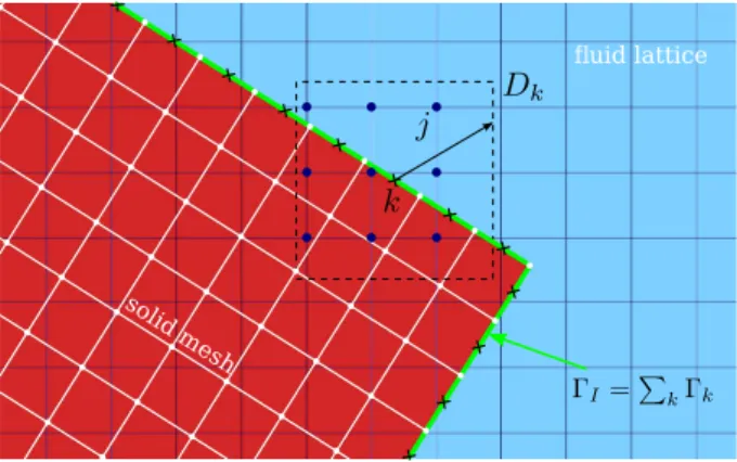
φ(xj, t)˜δ(xj−xk)∆x∆y (17) which provides an interpolated value of a given variableφ(x, t) at thekth solid pointxk =x(Xk, t) with Xk being the time-independent Lagrangian coordi- nate. This form of the interpolation operator makes use of the sampling property of the Dirac delta functionδ(x). In Equation (17),φ(xj, t) is the value ofφat thejth Eulerian (fluid) node located inside the support domainDk of the kth Lagrangian (solid) point, as shown in Figure 4. Finally, ˜δ(xj−xk) is a mollifier or a smooth approximation to the Dirac delta function. In the present work, we adopt the mollifier proposed by Roma et al. [33]:
˜δ(xj−xk) = 1
∆x˜δx
|xj−xk|
∆x 1
∆yδ˜y
|yj−yk|
∆y
(18) with:
δ˜x(r) = ˜δy(r) =
1 3
1 +p
−3r2+ 1
0≤r <0.5 1
6
h5−3r−p
−3(1−r)2+ 1i
0.5≤r <1.5
0 otherwise
(19)
where r denotes the nondimensional distance between the fluid node and the solid point in each direction, i.e. r=|xj−xk|/∆xorr=|yj−yk|/∆y.
Supposing that at the instanttnall variables are already known, and we will resolve the LB equation in order to update the fluid state to the instanttn+1. After calculating the new distribution functions fin+1 with Equation (11), we can update the fluid density by ρn+1f = P
ifin+1, but we cannot update the fluid velocity, since the IB-related body force F is not known yet. To clarify this point, let us rewrite Equation (16) at the instanttn+1:
Ih ρn+1f i
kvn+1f,k =I
"
X
i
cifin+1
#
k
+∆t
2 Fn+1k (20)
In one-way FSI problems, such as the ones presented in [22], the fluid velocity at the solid pointvn+1f,k is equal to the solid velocity under the no-slip condition,
solid m esh
uid lattice
Figure 4: The fluid lattice and the support domainDkofkthinterface point for IB method.
which is usually preset or imposed by the applied solid-motion law. As a result, one can directly calculate the IB-related forceFn+1k at solid points. However, in two-way FSI simulations, the velocityvn+1f,k can only be known after resolving the system of coupling equations, since the solid velocity at the instanttn+1also depends onFn+1k . That is why it is referred to as thetwo-way coupledproblem.
In the proposed FE-LB coupling method, vn+1f,k and Fn+1k will be obtained together by resolving a system of coupling equations, then the forceFn+1k will be spread from the Lagrangian (solid) points onto the neighboring Eulerian (fluid) nodes by means of the following spreading operation:
F(xj, t+ ∆t) = X
k∈Dj
Fn+1k ˜δjkn+1ǫn+1k ∆sn+1k (21)
where ˜δjkn+1= ˜δ(xn+1j −xn+1k ) andǫn+1k denotes the numerical width of thekth solid segment attn+1, which is obtained by resolving a linear system of equations in order to enforce the reciprocity of the interpolation-spreading operations [30, 12, 22]. Finally, ∆sn+1k is the length of the kth segment attn+1. Note that the use of the explicit Newmark scheme allows us to explicitly update the structural geometry so that we can calculate the ˜δjkn+1, ǫn+1k and ∆sn+1k independently of the coupling procedure within each time-step.
It is here noteworthy that in the present interpolation-based IB method for the FE-LB coupling, the LB equation is solved on all the lattice nodes, even for
the ones inside the solid domain. This allows us to apply the same treatment for all the lattice nodes and no special initialization technique is required for the freshly appeared real fluid nodes.
3. FE-LB coupling algorithm via an IB method
Physically, at the fluid-solid interface, there exist the continuities for the velocity and the force, respectively. However, this is not always true in the numerical simulations, due to the use of a straightforward or simple coupling algorithm. For example, when using FE method with Newmark time integrator for solid structure, the discrete system of equations for solid is given as:
Msan+1s =fextn+1−fintn+1 un+1s =uns + ∆tvsn+∆t2
2
(1−2β)ans + 2βan+1s vn+1s =vns+ ∆t
(1−γ)ans +γan+1s
(22)
where the external nodal force fextn+1, see Equation (8), depends on the dis- placement fieldun+1s and the flow-induced forceΛn+1 at the interface and next time-steptn+1. It is obvious that one cannot accomplish the time integration without knowingΛn+1.
In order to simplify the coupling procedure, one may assume that the flow- induced forceΛis constant during each time-integration step for the solid sub- domain and this force has the value at the previous instanttn, i.e. Λ = Λn for t ∈ (tn, tn+1]. With this assumption, fextn+1 can be calculated, so that the solid state can be updated to the next time-step. Then the fluid solver receives the updated solid geometry and velocity in order to finish the time integration.
This coupling procedure is referred to as the Conventional Serial Staggered (CSS) coupling algorithm [13].
As presented previously in Section 1, the CSS coupling algorithm might inject artificial or algorithmic energy into the coupled system, which sometimes causes numerical instability for the FSI simulation. The incremental interface energy∆EI can be used to measure the energy injection or dissipation at the
fluid-solid interface due to the staggered coupling algorithm. The definition of
∆EI is given as:
∆EI = X
k∈ΓI
Z tn+1 tn
Fs,k·vs,k dt+ X
k∈ΓI
Z tn+1 tn
Ff,k·vf,k dt (23) whereFs,k(orFf,k) is the interface force exerted on solid (or fluid), which can be calculated asFs,k=λk∆sk andFf,k=Fkǫk∆sk. vs,k(orvf,k) is the solid (or fluid) velocity at thekth interface element, as shown in Figure 4. Using the trapezoidal rule, one can approximately calculate ∆EI as:
∆EI ≃ X
k∈ΓI
∆tFs,k·vs,k
| {z }
Ws
+X
k∈ΓI
∆tFf,k·vf,k
| {z }
Wf
(24)
whereFs,k= (Fn+1
s,k +Fns,k)/2 andFf,k = (Fn+1
f,k +Fnf,k)/2 denote the mean values of the interface forces at the kth interface element, which act on the solid and the fluid, respectively. vs,k = (vn+1s,k +vns,k)/2 and vf,k = (vn+1f,k + vnf,k)/2 are the mean velocities of solid and fluid at the interface. Ws andWf
represent the external work transferred to the solid and fluid subdomains at the interface. Clearly, when the force and velocity continuity conditions are ensured, i.e. Fs,k(t) =−Ff,k(t) and vs,k(t) =vf,k(t) ∀t∈[. . . , tn−1, tn, tn+1, . . .] , the quantity of the incremental interface energy ∆EI = Ws+Wf is zero. Since the CSS algorithm cannot ensure the continuities at the interface, this quantity
∆EI is generally not zero with the CSS algorithm.
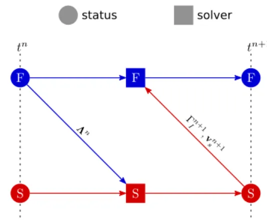
3.1. The CSS coupling algorithm
In order to show the importance of the interface-energy-conserving feature of the proposed coupling method, we provide a comparison with the CSS coupling algorithm in the context of FE-LB coupling simulation. The procedure of this staggered algorithm is illustrated in Figure 5 and can be briefly summarized as:
1 The interface force field Λn is sent to the solid solver, considered as the flow-induced force acted on the structure attn+1
2 Using this force boundary condition, the solid solver makes use of the Newmark time integrator (6) to update the solid status to the next instant tn+1: un+1s ,vsn+1,an+1s
3 Meanwhile, the fluid solver calculates the new distribution functionfin+1 by Equation (11) with the fluid statusfin,ρnf,vnf andFnknown from the previous time-step
4 The newly obtained structural geometry and velocity condition are sent to the fluid solver as a preset solid boundary condition, with which one will determine the new IB-related body forceFn+1 so as to fully update the macroscopic fluid status totn+1 with Equation (15): ρn+1f andvn+1f 5 Go to 1 for the next time-step
status solver
Figure 5: The Conventional Serial Staggered (CSS) coupling algorithm.
As one can observe, there is a time lag in this CSS coupling procedure, because the solid solver takes the interface force Λn as the force boundary condition at the instant tn+1. Such assumption ruins the force continuity at the fluid-solid interface, which is the main reason why such staggered coupling method suffers sometimes from numerical instabilities [23, 24, 26].
Given the definition of the incremental interface energy Equation (23) and Equation (24), one can evaluate ∆EI for the CSS coupling algorithm over one
time-step as follows:
∆EICSS= ∆t X
k∈ΓI
vs,k· Fn+1s,k +Fns,k
2 +Fn+1f,k +Fnf,k 2
!
(25) where we applied the velocity continuity condition vs,k(t) = vf,k(t), because in this CSS algorithm (Figure 5) the fluid and solid solvers share the same interface velocity. However, the interface force is not the same for the two solvers, because:
Fn+1
s,k =−Fnkǫn+1k ∆sn+1k Fn+1
f,k =Fn+1k ǫn+1k ∆sn+1k
(26) As a result, the value of ∆EICSS might have positive or negative value, corresponding to an algorithmic energy injection or dissipation, respectively, at the interface for the whole coupled system. As mentioned in the paper of Combescure and Gravouil [5], this interface energy condition is crucial in terms of numerical stability for the time integration of the coupled system.
Indeed, even if the individual schemes for solid and fluid subdomains are both numerically stable, the FSI simulation will still encounter instability issues when too much algorithmic interface energy is injected into the system.
Farhat and Lesoinne [9] has proposed an Improved Serial Staggered (ISS) coupling method which does not introduce errors of energy exchange at the fluid-solid interface. However, this method is not easy to be applied in the FE- LB coupling context, because neither the Newmark integrator nor the LB solver relies on the variable’s state at the mid-time-steptn+1/2.
3.2. The proposed non-staggered FE-LB coupling method
We shall provide here the details of the proposed non-staggered FE-LB cou- pling method via an IB scheme. As an implicit coupling procedure, it consists in resolving a system of coupling equations involving the solid and fluid equations, and the continuity conditions at the interface as well.
Starting with the solid coupling equations, let us write Equation (4) at the instanttn+1:
Msan+1s =fextn+1−fintn+1 (27)
Combining Equation (27) with the Newmark scheme (6) yields the solid equations that will be used in the coupling system:
Kcsvsn+1+Ln+1p Λn+1=gn+1s (28) where Ln+1p is the geometric operator constructed as previously described in Section 2.1,, which is based on the explicitly updated solid geometry with the chosen explicit Newmark scheme (β = 0 andγ= 0.5), andΛn+1is the interface force field attn+1. In addition,Kcsand gn+1s are calculated as:
Kcs= 2
∆tMs gsn+1=Ms
2
∆tvsn+ans
−fintn+1
(29)
Since the new displacement fieldun+1s has been calculated with the explicit Newmark scheme, one can then update the internal nodal force field with Equa- tion (4) and the Saint Venant-Kirchhoff material model. As a result, there are only two unknowns in Equation (28), which are vn+1s and Λn+1. Now, let us omit the n+ 1 superscript for the already calculated operator or matrix, i.e.
Ln+1p andgn+1s , so that we can rewrite Equation (28) as:
Kcsvn+1s +LpΛn+1=gs (30) As for the fluid coupling equations, by multiplying Equation (20) with the numerical local widthǫn+1s of thekth IB-segment, we can obtain:
2ǫn+1k
∆t Ih ρn+1f i
kvn+1f,k −ǫn+1k Fn+1k =2ǫn+1k
∆t I
"
X
i
cifin+1
#
s
(31)
where−ǫn+1k Fn+1k =λn+1k represents the interface force per unit length exerted on the solid at thekth interface element or segment. Once again, let us omit then+ 1 superscript for the already known variables and rewrite Equation (31) in matrix form as:
Kcfvn+1f +Λn+1=gf (32)
with:
Kcf=
Kcf,1 0 . . . 0 0 Kcf,2 . . . 0 ... ... . .. ... 0 0 . . . Kcf,N
k
,vn+1f =
vn+1f,1 vn+1f,2
... vn+1f,N
k
andgf =
gf,1 gf,2 ... gf,Nk
(33)
where, for thekth segment, we have:
Kcf,k= 2ǫn+1k
∆t Ih ρn+1f i
kI gf,k= 2ǫn+1k
∆t I
"
X
i
cifin+1
#
k
(34)
Now we have the solid and fluid coupling equations (30) and (32) with the unknown vn+1s , vn+1f and Λn+1. Obviously, one more equation is needed to solve the coupling system, which will come from the velocity continuity condition under the no-slip condition at the fluid-solid interface:
Lsvn+1s +vn+1f =0 (35) where Ls is another geometric operator that gives the solid velocity at the interface from the velocity fieldvs.
Regrouping the equations (30), (32) and (35) gives the coupling system of equations:
Kcs 0 Lp 0 Kcf I Ls I 0
vsn+1 vfn+1 Λn+1
=
gs gf 0
(36)
To solve such system of equations, we follow the procedure presented in [5, 24]:
(1) Calculate thefreevelocities by:
vf rees = [Kcs]−1gs andvf reef = Kcf−1
gf (37)
(2) Calculate the condensed matrix H, which is essentially the Poincar´e- Steklov operator:
H=Ls[Kcs]−1Lp+ Kcf−1
(38)
(3) Calculate the interface force fieldΛn+1 at the instanttn+1: Λn+1=H−1n
Ls[Kcs]−1gs+ Kcf−1
gf
o (39)
(4) Calculate thelinkvelocities:
vlinks =−[Kcs]−1LpΛn+1 andvlinkf =− Kcf−1
Λn+1 (40) (5) Finally, regroup thefreeandlinkvelocities in order to get the totalveloc-
ities:
vn+1s =vsf ree+vlinks andvn+1f =vf reef +vlinkf (41) Once Λn+1, vsn+1 and vn+1f are updated, the solid solver will use vn+1s to calculate the new acceleration field through Equation (6) withγ= 0.5. Mean- while, the fluid solver will spread this newly obtained interface force fieldFn+1 from the solid points onto the neighboring fluid nodes in order to accomplish the calculation of the macroscopic fluid velocity by Equation (15).
It is worth noting that in Equation (36) the matrixKcs,Kcf,Lp andLsare all independent of the unknownsvn+1s ,vn+1f andΛn+1, due to the use of explicit Newmark time integrator. It can then be easily demonstrated that the present resolution procedure is mathematically equivalent with a direct one. This lin- earity allows us to split the final velocity solution field into two parts: the free velocity and the link velocity, so that the fluid and solid solvers can calculate first their free velocities individually and simultaneously. In addition, instead of directly solving the system of equations (36), we solve the condensed equation (38) which has a much smaller dimension than Equation (36). All these make the present resolution procedure very efficient.
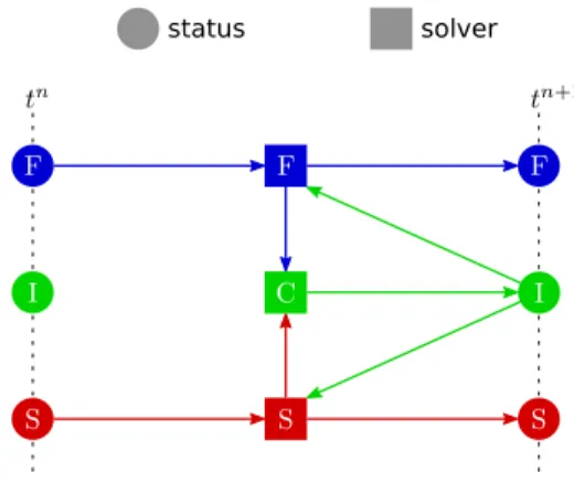
Now, the proposed coupling algorithm is illustrated in Figure 6, and can be briefly reviewed as follows:
1 The solid and fluid solvers carry out independently and simultaneously the first-stage calculation: the solid solver calculates the new displace- ment fieldun+1s using the explicit Newmark scheme and then update the
structural geometry; the fluid solver carries out the collision and streaming steps of LB method so that one can update the fluid densityρn+1f 2 The coupler interpolates the fluid information shown in Equation (20)
from the fluid nodes to the newly updated solid points so as to prepare Kcf and gf, and then receives Kcs and gs from the solid solver in order to obtain the Λn+1, vn+1s and vn+1f by resolving the coupling system of equations (36)
3 The solid solver receives vn+1s and the fluid solver receives Λn+1 from the coupler and then accomplish the individual integrations of one entire time-step
status solver
Figure 6: The proposed implicit strong coupling algorithm (F, S, I and C correspond to ‘Fluid’,
‘Solid’, ‘Interface’ and ‘Coupler’, respectively).
4. Numerical validations and discussions
In this part, we have adopted a widely used numerical test case [2, 19, 35, 36, 37] to validate the present FE-LB coupling method. Before showing the FSI results, we provide two numerical validations for the solid and fluid solvers alone.
Finally, the FSI results are shown and the stability of the proposed algorithm is discussed.
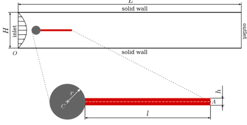
4.1. Configuration of the numerical test case
This well-known test case was firstly proposed by Turek and Hron [37] for the numerical benchmarking of laminar flow-elastic structure FSI simulations.
As shown in Figure 7, we consider an elastic solid bar immersed in a rectangular fluid flow channel. The deformable solid bar is attached to a fixed rigid cylinder, of which the geometric center is located near the inlet and slightly deviated from the horizontal center line of the channel. The geometric and material parameters are provided in Table 1 and Table 2, respectively.
inlet
solid wall
solid wall
outlet
Figure 7: Configuration of the validation test case.
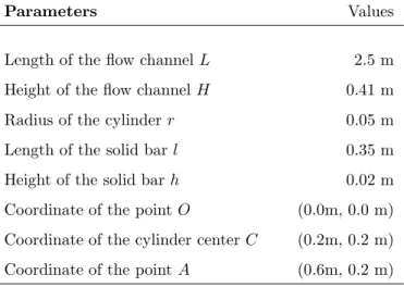
Table 1: Geometric parameters of the FSI test case.
Parameters Values
Length of the flow channelL 2.5 m
Height of the flow channelH 0.41 m
Radius of the cylinderr 0.05 m
Length of the solid barl 0.35 m
Height of the solid barh 0.02 m
Coordinate of the pointO (0.0m, 0.0 m) Coordinate of the cylinder centerC (0.2m, 0.2 m) Coordinate of the pointA (0.6m, 0.2 m)
At the inlet of the flow channel, a parabolic velocity profile is imposed by:
vfx(0, y) = 1.5Uy(H−y) (0.5H)2 vyf(0, y) = 0
(42)
whereU = 1 m/s denotes the spatially mean inlet velocity, which will be used to determine the Reynolds number Re =U D/νf = 100 with D and νf being the diameter of the fixed cylinder and the kinematic fluid viscosity, respectively.
Additionally, no-slip boundary conditions are applied at the upper and lower solid wall. All these three velocity boundary conditions are ensured by means of the scheme of Zou and He [40] for the LB simulation.
As for the outflow boundary condition, we apply a linear extrapolation scheme [25] for the distribution functions fi for i ∈ [1,8], while tuning the f0 in order to impose a prescribed exit density or pressure value. As a conse- quence, we can linearly extrapolate the fluid velocity and fix the fluid density to a certain value at the outlet.
Initially, the whole field is at rest and a smooth increase of the inlet velocity is imposed as:
vfx(0, y, t) = 1.5Uy(H−y) (0.5H)2
1−cos(0.5πt)
2 ift <2.0 s vfx(0, y, t) = 1.5Uy(H−y)
(0.5H)2 otherwise
(43)
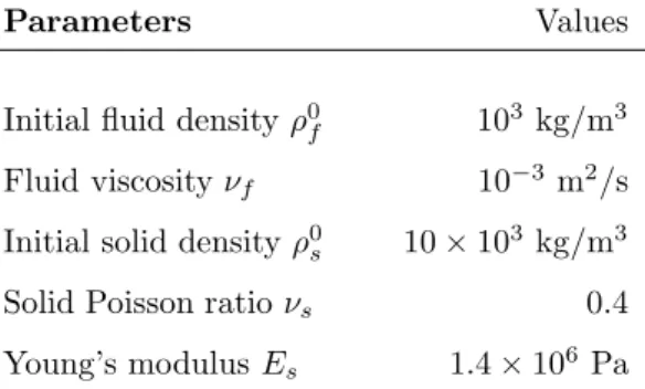
Table 2: Material parameters of the FSI test case.
Parameters Values
Initial fluid densityρ0f 103kg/m3 Fluid viscosityνf 10−3m2/s Initial solid densityρ0s 10×103kg/m3
Solid Poisson ratioνs 0.4
Young’s modulusEs 1.4×10⁶ Pa
The fluid subdomain is discretized with a uniform lattice of size 1250∆x× 205∆ywith ∆x= ∆y. As the LB equations are usually resolved with dimension-
less variables, we choose thelengthrescaling factor Cx = ∆xp/∆xl = 0.002 m and thetimerecaling factorCt= ∆tp/∆tl= 10−4 s so that the lattice spacing
∆xl= 1 and the lattice time-step ∆tl= 1, where the superscriptspand l are devoted tophysicalandlattice, respectively. Hence, the velocity rescaling factor is determined asCv = ∆xp/∆tp = 20 m/s. As a result, the lattice mean inlet velocity, the speed of sound in fluid, the viscosity and the relaxation time can be calculated by Ul = Up/Cv = 0.05, cls,f = p
1/3, νfl = UlDl/Re = 0.025 and τl = 3νfl + 0.5 = 0.575, respectively. Note that in such case we have a small Mach numberM a=Ul/cls,f ≃0.0288≪1, which is consistent with the incompressible limit for the adopted LB model.
Here it is worth noticing that in the present work the solid mesh and the IB frontier have the same spacing as the fluid lattice, i.e. ∆X = ∆s = ∆x.
Additionally, the fluid and solid solvers use the same time-step. Hence, given the material parameters in Table 2, one can estimate the critical time-step for the solid solver with Equation (7) as ∆tcrit = ∆xp/p
Es/ρ0s ≃ 1.69×10⁻⁴ s, which is larger than the used time-step ∆tp= 10−4 s.
One may observe that the time-step is quite restricted. This is mainly due to two reasons. First, we use here the explicit Newmark time integrator for the solid structure. While this choice allows us to explicitly calculate the solid displacement attn+1 without subiterations, it does limit the time-step because of its explicit feature as time integrator. Second, in the present work, we use the identical time-step for the solid and fluid solvers. In addition to this, the time-step ∆t and the space-step ∆x are tied up for LB solver. Consequently, one needs to choose the same time-step which should be appropriate for the solid as well as for the fluid solvers.
4.2. Validations of the solid and fluid solvers
Before coupling the fluid and solid subdomains, it is necessary to validate individually the solid and fluid solvers using some pure solid and pure fluid test cases.
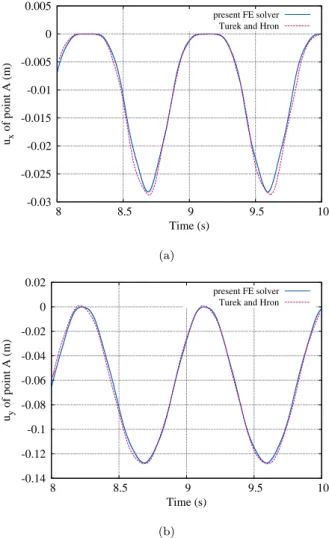
To do so, we have carried out firstly a pure solid test case, in which the solid
bar is only charged by the gravity body force. It corresponds to the “CSM3”
test case proposed by Turek and Hron [37], whereg =−gez withg = 2 m/s2 andρ0s= 103 kg/m3. The other material parameters are the same as in Table 2. Figure 8 shows the time evolution of the displacement of the point A (see Figure 7) in x- and y-directions. A good agreement with the results of Turek and Hron [37] can be found in Figure 8, which allows us to validate the present FE solver in such kind of configuration for the solid simulation.
-0.03 -0.025 -0.02 -0.015 -0.01 -0.005 0 0.005
8 8.5 9 9.5 10
ux of point A (m)
Time (s)
present FE solver Turek and Hron
(a)
-0.14 -0.12 -0.1 -0.08 -0.06 -0.04 -0.02 0 0.02
8 8.5 9 9.5 10
uy of point A (m)
Time (s)
present FE solver Turek and Hron
(b)
Figure 8: Time history of the point A’s displacement in x- and y-directions.
Secondly, we also validate the present LB solver with a steady test case
(“CFD2” in [37]) by measuring the drag and lift on the fixed and rigid cylinder- bar entity in the flow channel under the previously presented fluid boundary conditions. In Table 3, one can observe that the steady drag and lift obtained by the present LB solver are in good agreement with the ones in [37]. A difference less than 3% is found between the two results, which validates the present LB solver for fluid simulation. More validations for the LB solver can also be found in the previous work [22] of the authors.
0 20 40 60 80 100 120 140 160 180
0 5 10 15 20 25 30 35 40 45 50
Drag and lift (N)
Time (s)
140.6
10.8
Re = 100
Drag Lift
Figure 9: Drag and lift in the steady pure fluid test case.
Table 3: Drag and lift in the steady fluid solver validation test case.
Drag (N) Lift (N) Present method 140.6 10.8 Turek and Hron [37] 136.7 10.5
Difference 2.85% 2.86%
4.3. Numerical results of the FSI simulations
4.3.1. Results with the proposed synchronous FE-LB coupling method
Now, we shall present the FSI results obtained with the proposed syn- chronous FE-LB coupling method. Figure 10 shows the vorticity fieldωf in the fluid flow and the stress component σsxx in the solid bar at different instants.