HAL Id: hal-00624984
https://hal.archives-ouvertes.fr/hal-00624984v1
Submitted on 20 Sep 2011 (v1), last revised 28 Jan 2013 (v2)
HAL is a multi-disciplinary open access archive for the deposit and dissemination of sci- entific research documents, whether they are pub- lished or not. The documents may come from teaching and research institutions in France or abroad, or from public or private research centers.
L’archive ouverte pluridisciplinaire HAL, est destinée au dépôt et à la diffusion de documents scientifiques de niveau recherche, publiés ou non, émanant des établissements d’enseignement et de recherche français ou étrangers, des laboratoires publics ou privés.
State-based accelerations and bidirectional search for bi-objective multimodal shortest paths
Christian Artigues, Marie-José Huguet, Fallou Gueye
To cite this version:
Christian Artigues, Marie-José Huguet, Fallou Gueye. State-based accelerations and bidirectional search for bi-objective multimodal shortest paths. 2011. �hal-00624984v1�
State-based accelerations and bidirectional search for bi-objective multimodal shortest paths
Christian Artigues1,2,Marie-Jos´e Huguet1,2, Fallou Gueye1,2,3
1CNRS ; LAAS ; 7 avenue du colonel Roche, F-31077 Toulouse Cedex 4, France
2Universit´e de Toulouse ; UPS, INSA, INP, ISAE ; UT1, UTM, LAAS ; F-31077 Toulouse Cedex 4, France
3MobiGIS; ZAC Proxima, rue de Lannoux, 31310 Grenade Cedex France artigues@laas.fr, huguet@laas.fr
Abstract
Taking into account the multimodality of urban transportation networks for com- puting the itinerary of an individual passenger introduces a number of additional constraints such as mode restrictions and various objective functions. In this paper, constraints on modes are gathered under the concept of viable path, modeled by a non deterministic finite state automaton (NFA). The goal is to find the nondominated viable shortest paths considering the minimization of the travel time and of the num- ber of modal transfers. We show that the problem, initially considered by Lozano and Storchi [15], is a polynomially-solvable bi-objective variant of the mono-objective regular language-constrained shortest path problem [2, 8].
We propose several label setting algorithms for solving the problem: a topological label-setting algorithm improving on algorithms proposed by Pallottino and Scutell`a [23] and Lozano and Storchi [15], a multi-label algorithm using buckets and its bidirec- tional variant, as well as dedicated goal oriented techniques. Furthermore, we propose a new NFA state-based dominance rule. The computational experiments, carried-out on a realistic urban network, show that the state-based dominance rule associated with bidirectional search yields significant average speed-ups. On an expanded graph comprising 1 859 350 nodes, we obtain on average 3.5 nondominated shortest paths in less than 180 ms.
keywords: bi-objective regular language-constrained shortest path problem, mul- timodal transportation, finite state automaton, label-setting algorithms, state-based dominance rule, bidirectional search, state-based estimated travel times.
1 Introduction
Computing shortest paths in the context of monomodal passenger transportation, where a single transportation mode (e.g. private vehicle, bus, subway) is used during the pas- senger’s itinerary, has been the subject to extensive research since the publication of Dijkstra’s algorithm in the 1950s. Among the considered extensions of the basic shortest path problem, the case where travel times (or costs) are time-dependent, allowing to take into account public transportation timetables or traffic congestion hours, has also been
widely studied. Nowadays, thanks to powerful acceleration and/or preprocessing tech- niques (such as bidirectional search, A∗ search, landmarks, contraction hierarchies, etc.), computing shortest-paths very fast in large-scale network, either in a time-independent or in a time-dependent context, is not a challenge anymore for labeling algorithms [6, 7, 19].
The case of multimodal passenger transportation, which lies in the transportation of one or several passengers with different modes during the same itinerary, has been much less addressed. However, multimodal transportation is subject to a growing interest in the research community, as multimodality is now widely accepted for urban transportation as a necessary alternative to the exclusive use of private vehicles.
In this paper, we consider a bi-objective shortest path problem in a multimodal urban transportation network: the minimum travel time/minimum number of transfers regular language-constrained shortest-path problem, initially considered by Lozano and Sorchi [15], and denoted by BI-RegL-CSPP by analogy to its mono-objective variant: the regular language (or label)-constrained shortest path problem RegL-CSPP defined by Barett [2] and recently considered in [1, 8, 22]1.
The problem can be briefly stated as follows. Given a networkG(V, E) in which each node i ∈ V is “colored” by a mode mi (e.g. bus, walk, car, subway) and each arc from i∈ V is weighted by a travel time distance which corresponds to a travel time in mode m if mi = mj = m or to a transfer time if mi 6= mj. Furthermore, there are so-called path viability constraints. More precisely, the sequence of modes induced by a path is constrained in such a way that the string obtained by concatenating the path modes (considered as elements of an alphabet) must belong to a formal language described by a non-deterministic finite state automaton (NFA). Considering an origin node O and a destination nodeD, the goal is to find anO−Dpath for each of the nondominated points in the space of two min sum objectives: the minimum total travel time and the minimum number of transfers (mode changes along the path). As in [15], we restrict ourselves to a time-independent version of the problem (travel times are constant) but we will briefly describe an extension scheme of the proposed algorithms to FIFO networks in Section 7.
Lozano and Sorchi [15] implicitely assume (without mentioning it) that the problem can be solved in polynomial or pseudo-polynomial time. They proposed a label correcting algorithm to solve the problem, based on a topological labeling algorithm proposed by Pallottino and Scutell`a in [23].
In this paper we first prove the problem can actually be solved in polynomial time.
We propose a label setting extension of the Pallottino and Scutell`a algorithm and sev- eral improvements to the Lozano and Sorchi approach, among which a new state-based dominance rule. We also propose a multi-label approach based on buckets, from which we derive a bidirectional label setting algorithm. Goal-oriented techniques with state- dependent estimated travel times are finally presented. We consider an application to the urban area of Toulouse (France), the purpose of which being to evaluate the tractability of the considered problem on a real-life network, as no computational experiments were reported in [15]. On this practical network, we compare the different algorithms. In par- ticular we study the impact of the dominance rules and the impact of the size and nature of the NFA on the CPU time and on the number of touched nodes.
Section 2 briefly recalls the existing literature on the multimodal shortest path problem, so as to introduce our motivations for the present study. Section 3 formally defines the problem. The proposed algorithms are presented in Section 5. Their performance on the
1Lozano and Storchi [15] referred to the problem as the multimodal viable shortest-path problem
considered real network are compared in Section 6. Further extensions and concluding remarks are presented in Section 7.
2 Literature review
Multimodal transportation raises network modeling issues [5, 14]. A simple way of model- ing the network, used by many authors [18, 15, 4], lies in assuming that the set of nodes is partitioned according to the modes. An arc linking two nodes of different subsets is called a transfer arc. Equivalently, nodes and/or arcs are labeled according to the associated mode [2]. Once such a network is defined, one typically seeks to model the fact that some sequences of modes constituting a path can be infeasible in practice. A first (relaxed) way of taking account of such mode restrictions for shortest path computations was proposed by Modesti and Sciomachen [18], as an extension of Dijkstra’s algorithm to minimize a (single) global utility function defined by a weighted sum of modal characteristics of a path (time spent on the private car, time spent on the bus or subway, walking time, waiting time,...). For shortest path computation including hard modal constraints, (possibly infi- nite) mode-dependent travel times were used by Ziliaskopoulos and Wardell [27], together with an arc representation, allowing to design mode constraints involving three nodes. A more general way of modeling the multimodal constraints (among other applications) was proposed by Barettet al.[2]. Each mode being viewed as an element of an alphabet, each arc of the network being labeled by a mode, the mode restrictions can be described by a regular language over the alphabet. The multimodal shortest path problem then amounts to a regular language-constrained shortest path problem (RegL-CSPP). As a regular language can be represented by a non-deterministic finite state automaton (NFA), Barett et al.[2] proved that the problem is polynomial in the number of states of the automaton.
In [1, 8, 22, 26, 25], practical implementation issues of this method have been discussed.
Barett et al.[1], proposed A∗ and bidirectional accelerations while Delling et al. [8] and Pajor [22] proposed, in addition, core-based and access node-based speed-up techniques and also considered time-dependent networks. With these techniques, they obtain a CPU time of 2.3 milliseconds on average for computing the O−D shortest path on a large intercontinental network with 50 700 647 nodes, 125 939 503 edges, a 3 state-automaton.
Considering deterministic finite-state automaton (DFA) as input, Sheraliet al.[25] extend the problem to time-dependence and propose a strongly polynomial algorithm for FIFO graphs. Sherali and Jeenanunta [26] further extend the problem to approach-dependent travel times and propose a label-setting algorithm which consistently outperforms a label correcting algorithm designed for the same problem.
The main drawback of the approaches based on the RegL-CSPP are that they all consider only a single objective. However, when several modes are available, a user may want to select her/his itinerary among a set of alternatives, taking account of several objectives. To that purpose, two general classes of multi-objective multimodal shortest path problems have already been considered in the literature: namely, (pseudo-)polynomial problems and NP-hard problems.
Pallottino and Scutell`a considered in [23] the Bi-RegL-CSPP problem without the viability constraints (anyO−Dpath is feasible) but with the constraint that the number of transfers does not exceed a maximum numberkmax. Although the general bi-objective shortest path problem with min-sum objective is NP-hard, they showed that, in this case, the problem can be solved in pseudo-polynomial time (in n, the number of nodes in the network, and kmax), as it belongs to the category of bi-objective shortest path problems
for which one of the two objectives takes its values in a discrete and finite set. They proposed a topological labeling approach where a label (i, k) represents anO−ipath with ktransfers.
In [15], Lozano and Storchi directly extended this problem and the topological algo- rithm, so as to integrate mode restrictions using a NFA in a time-independent network, defining theBi-RegL-CSPP considered in the present paper. Note they performed this extension without formally proving that the problem is (pseudo-)polynomial. We will prove in the sequel that the problem can actually be solved in polynomial time in nand
|S|, the number of states of the NFA.
Bielli et al [4] considered a simplified version of the NFA model but include time- dependent arcs and time penalties for turning movements. Their objective is to compute theK−shortest paths under an upper bound of the maximum allowed number of trans- fers. The method can also be defined as an extension of the topological Pallottino and Scutell`a [23] algorithm, with labels on arcs. Experimentations are limited to small net- works. The largest one, presented in [4], involves 1000 nodes and 2830 arcs and the K-shortest path algorithm runs in 6.5s on a Pentium II with 64 MB RAM. To our knowl- edge, no realistic computational experiments were carried out for the Bi-RegL-CSPP. Besides providing new algorithms and acceleration techniques, our main purpose in this paper is consequently to study the tractability of solving this bi-objective problems on a real network in reasonable computational time.
A more general class of approaches considers several different objective functions and, mostly, proposes extensions to multimodality of the (NP-hard) bi-objective shortest path problem. Although we focus in this paper on the polynomial Bi-RegL-CSPP, we men- tion the recent experimental study carried out by Gr¨abeneret al.[10] for a more general problem since the number of transfers and minimum time objectives were also considered among other objectives in their study. They present an extension of Martin’s algorithm [17]
to deal with the multimodal, multiobjective shortest path problem, considering only ba- sic mode restrictions (the finite state automaton formalism is not used). When only the minimum number of transfers and minimum time objectives are considered, the method shows very fast computational times. For three modes (cycling, walking and public trans- portation), in a time-dependent context, the pareto-optimal paths are computed in 71.9 milliseconds in average for a network of 36694 nodes and 171443 edges. However the num- ber of nondominated paths is on average equal to 1.2. Actually, since the cycling mode can be taken from the origin to the destination (or left anywhere in the network), it generally dominates the other modes. This recent study partially answered our question in the sense that they showed that the bi-objective multimodal problem is actually tractable when no complex mode restrictions are defined and when one of the modes tends to dominate the others.
In this paper we propose specific algorithms for theBi-RegL-CSPPand we evaluate the practical tractability of real instances admitting significantly more nondominated so- lutions and where complex mode restrictions are represented by a finite state automaton.
Furthermore, we evaluate the efficiency of a new NFA state-based dominance rule and of a new bidirectional label-setting algorithm based on buckets.
3 Problem statement
3.1 Definition
LetM denotes the set of modes. The multimodal transportation network is modeled by a multi-layered networkG(V, E) with|V|=nsuch that each layer corresponds to a mode m∈M. Hence, a mode mi ∈M is defined for each node i∈V while a travel timedij is associated to each arc (i, j)∈E. An arc (i, j) such thatmi6=mj is called a transfer arc.
In terms of multimodal characteristics, each path in Gyields a sequence (or string) of modes. Among all strings of modes, only a subset of strings are acceptable according to the feasibility constraints (or to passenger’s preferences). The acceptable mode sequences are represented via a non-deterministic finite state automaton (NFA), possibly issued from a user-defined regular expression [2]. This NFA is given by a 5-uple A = (S, M, δ, s0, F) whereS={1, . . . ,|S|}is the set of states,s0 is the initial state,F is the set of final states and δ :M ×M ×S → 2S is the transition function such thatδ(m, m′, s) gives the set of states obtained when traversing, from state s, an arc (i, j) with mi = m and mj =m′. We assume that δ(m, m′, s) = ∅ denotes the case where the transition is infeasible. Note that the case wereδ(m, m′, s) is either the empty set or a singleton yields a deterministic finite state automaton (DFA).
A viable path is a path inGfrom an origin nodeOto the destination nodeDsatisfying the constraints represented by the NFA. A path is viable if it starts with O (in state s0) and reaches Din a final states∈F.
We consider both the “minimum time” and “minimum number of transfers” objectives.
We first recall definitions on multi-objective optimization [9] applied to our problem. Let time(p) denote the travel time along a pathp. Letntr(p) denote the number of transfers along p. An efficient (or Pareto-optimal) solution is a feasible O-D path p such that there is no other path p′ verifying either time(p′) ≤ time(p) and ntr(p′) < nbtr(p), or time(p′)< time(p) andntr(p′)≤nbtr(p). In the objective space, a nondominated point is a pair (t, k) such that there exists an efficient pathpverifyingtime(p) =tandntr(p) =k.
Considering the bi-objective “minimum time” and “minimum number of transfers”
O-D viable path problem, the goal is to find all nondominated points, and, for each of them, a single efficient path.
3.2 NFA scenarios
For our experimental evaluation on a real network, we consider 4 modes{w, b, c, s}(walk- ing, bus, private car, subway) and 3 different mode configuration scenarios: M1 ={w, b}
(walk and bus only), M2 = {w, b, s} (walk, bus and subway only) and M3 ={w, b, c, s}
(all modes).
For modeM3, we consider the constraint scenario used in [15]. The private car can be taken only fromO and, once left, cannot be taken again. For the subway, we assume that it can be taken at any time but, once left, cannot be taken again, which corresponds to a user preference.
These viability constraints are modeled by a NFA2 proposed by Lozano and Storchi [15] with|S|= 5 represented in Figure 1. Transition arcs between states are labeled by a modem∈M whereM ={w, b, c, s} ∪ {mO},mObeing a fictitious mode labeling only the originO. A transition from state sto states′ labeled bym∈M describes the transition
2The original NFA included a transition froms0 to s4 that we omitted since for our experiments, the origin nodes are never located in the subway
function of a traversed arc (i, j) in such a way that s′ ∈δ(mi, mj, s) with mj =m. If a modemdoes not appear as a possible transition of a given state s, any transition towards this mode is forbidden.
s0 start
s1
s2
s3
s4 s5
w, b c
w, b
s c
w
w, b s
w
s w, b
Figure 1: Original NFA for mode set M3={w, b, c, s}
The state at origin is denoted s0 and other states have the following meaning:
• s1: private car was not taken at the origin O and, so, mode c is forbidden for the remaining of the travel, while subway has not been taken yet;
• s2: private car was taken at the origin O and has not been left yet;
• s3 private car cannot be taken anymore since it has already been taken and left while subway mode has not been taken yet;
• s4: subway has been taken but not left;
• s5: subway has been left.
We consider that the acceptable final states are reduced toF ={s1, s3, s5}(displayed in double circle in Figure 1). Indeed, state s4 models the presence of the user in the subway, so she/he must leave the subway to reach her/his destination. State s2 means the private car is currently being used and must be left in a parking area to reach the destination. For mode set M2, as the car is not considered anymore, states s2 and s3 are removed and only 3 states remain in the NFA (see Figure 2(b)). For mode set M1, as there are no constrained modes anymore, the NFA is empty. Note that all considered input NFAs are also DFAs.
3.3 Example of Bi-RegL-CSPP
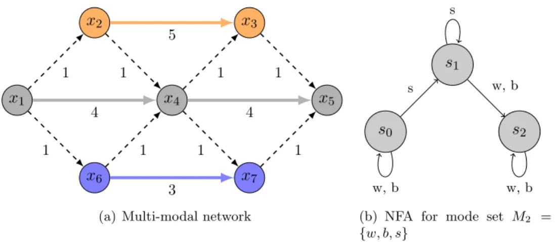
Figure 2(a) shows an (unrealistic) multi-modal network with 7 nodes corresponding to mode setM2 ={w, b, s}. Nodesx2 andx3 are bus (b) nodes; nodesx1,x4 andx5are walk (w) nodes; nodes x6 and x7 are subway (s) modes. Dashed arcs correspond to transfer arcs. The NFA corresponding to M2 is displayed in Figure 2(b).
x1 x4 x5
x6 x7
x2 x3
4 4
5
3
1 1 1 1
1 1 1 1
(a) Multi-modal network
s0
s1
s2
s
w, b
s
w, b
w, b (b) NFA for mode set M2 = {w, b, s}
Figure 2: aBi-RegL-CSPPwith 7 nodes, 12 arcs, 3 modes and a 3 state-NFA There are three non dominated solutions to the Bi-RegL-CSPP from x1 tox5: the first solution (x1, x4, x5) with 0 transfer and a travel time equals to 8, the second solution (x1, x6, x7, x5) with to 2 transfers and a travel time of 5 and the third one (x1, x2, x4, x3, x5) leads to 4 transfers and a travel time equals to 4. Note the pathx1, x6, x4, x7, x5 of cost 4 is infeasible as the automaton, initially in states0, is set tos1 taking transfer arc (x1, x6) and then to s2, through transfer arc (x6, x4) from which it is not possible to take the subway anymore.
4 Complexity
In this section we establish the complexity status of theBi-RegL-CSPP which was not stated in [15] although it was implicitly considered that the problem is pseudo-polynomial innandkmax(the maximum number of transfers). This seems intuitively correct. Indeed, Barett [2] proved that the mono-objective RegL-CSPP is polynomially solvable, while Pallottino and Scutell`a showed that the bi-objective minimum time/minimum number of transfers multimodal shortest path problem (without viability constraints) is pseudo- polynomially solvable under a thresholdkmax on the number of transfers.
Theorem 4.1. The Bi-RegL-CSPP can be solved in a time polynomial inn|S|.
Proof. Suppose in a first step that the number of transfers must not exceed a threshold kmax. We build an expanded graph by creating a node per tuple (i, s, k) for i ∈ V, s∈S,k∈ {0,1, . . . , kmax}and an arc from node (i, s, k) to (j, s′, k′) valuated by dij where (i, j)∈E, s′ ∈δ(mi, mj, s) andk′ =kifmi=mj and k′ =k+ 1 if mi 6=mj. By solving the single-source, multi-destination mono-objective shortest path problem in this graph from node (0, s0,0) (e.g. with Dijkstra’s algorithm) we obtain all nondominated solutions, simply by scanning the shortest paths ends (D, s, k) for s ∈F and k ∈ {0,1, . . . , kmax}.
This statement is a straightforward extension of the proof proposed by Barett [2] for the RegL-CSPP.
As the number of nodes in the expanded graph is equal to n|S|kmax, we just showed that the problem is pseudo-polynomially solvable. Consider now a nondominatedO−D path inG(V, E). We claim that the number of times this path visits a given node iis not larger than |S|, the number of states of the NFA. Indeed, suppose the path visits twice a nodei in states, i.e from node (i, s, k) to node (i, s, k′) of the expanded graph. then the
subpath (i, s, k), . . . ,(i, s, k′) can obviously be removed without increasing the number of transfers and the travel time nor violating the viability constraints, which contradicts the assumption that the path is nondominated. It follows that kmax cannot be larger than n|S|and so the above-described algorithm is polynomial in nand |S|.
Note that setting kmax to a number lower thann|S|accelerates the search and corre- sponds to a reasonable restriction in most applications.
5 Algorithms
In this section, we propose several algorithms and a new state-based dominance rule to solve the Bi-RegL-CSPP. All algorithms are based on a label setting principle which is described in Section 5.1. The dominance rules are presented in Section 5.2. The first al- gorithm (TLS), a label-setting version of the topological label algorithm proposed by [15]
with additional corrections and improvements, is given in Section 5.3. The second algo- rithm (MQLS), described in Section 5.4, is a new label setting algorithm based on buckets.
Section 5.5 presents the third algorithm (FB-MQLS), a bidirectional (Forward-Backward) adaptation of MQLS. Finally, Section 5.6 presents state-based goal oriented (A*) tech- niques for the unidirectional algorithms.
5.1 Label setting principle
The proposed algorithms use labels to represent paths. Let (i, s, k) denote a label repre- senting a path from the origin to nodeiin statesand usingktransfers. Each label has two attributes: tkis which denotes the arrival time on iand pkis which denotes the predecessor label of (i, s, k) on the path. Note that no algorithm needs to store more than one label (i, s, k) for given i,sand k.
All the proposed algorithms implement differently the following basic principles. Ini- tially, a label (O, s0,0) is generated with t0Os0 = 0 and p0Os0 = (O, s0,0). The label is stored in a convenient data structure Q. The label setting process is then applied until Qbecomes empty. At each iteration, the label (i, s, k) with minimum tkis is removed from Qand marked-up, as tkis is the shortest time from O toiin state swith ktransfers. Let M arkisk ∈ {true, f alse} denote the mark indicator and let M denote the set of marked nodes. Then, the direct successors of nodeiare scanned. For each successorj, viability of the arc (i, j) is checked according to multimodal restrictions and obtained labels (j, s′, k′) are considered for alls′ ∈δ(mi, mj, s),k′ =k ifmi =mj ork′ =k+ 1 if mi 6=mj. If one of the three following conditions, i.e.
(i) label (j, s′, k′) was never visited;
(ii) the Bellman condition does not hold (tkjs′′ > tkis+dij);
(iii) dominance rules do not apply (see Section 5.2),
the time and predecessor of (j, s′, k′) are updated with tkjs′′ ←tkis+dij and pkjs′′ ←(i, s, k) and the label is inserted in Q or, if it is already present, Q is updated according to tkjs′′
decrease. Otherwise the label is discarded.
5.2 Dominance rules and state reduction
In this section we give dominance rules allowing to discard labels. During the extension process, a label can be discarded if it can be proven that he cannot be extended to a better solution than another already generated label .
A first dominance rule, the basic dominance rule, is linked to the bi-objective optimiza- tion. It was used by Pallottino and Scutell`a in [23] to solve the bi-objective multimodal shortest path without viability constraints.
Proposition 5.1(Basic dominance rule). Consider two distinct labels(i, s, k)and(i, s, k′).
If k≤k′ andtkis ≤tkis′, label(i, s, k′) can be discarded (because it is dominated by the label (i, s, k)).
Enforcing this dominance rule yields only different solutions: if there are two solutions with same travel times and same numbers of transfers, only one of them is kept. This first dominance rule compares, for a given node, only labels having the same state.
The second dominance rule allows to go further by comparing, for the same node i, labels having different states. For that, we consider a binary relationon the states such thatss′ means that syields more extension possibilities thans′. More precisely, Definition 5.1. State sdominates state s′ (ss′) if any input mode string accepted by s′ is also accepted by s.
Lozano and Storchi already proposed such a dominance rule in [15] (Preference theo- rem). Unfortunately, we show that their rule applies to the NFA they consider (displayed in Figure 1) but does not hold in general. We recall below the Lozano and Storchi Theo- rem3.
Theorem 5.1 ([15]). State su is preferred to state sl, su sl, if the following sentences are valid:
(a) the constrained modes used in state su path, are a subset of the set of constrained modes used in state sl path;
(b) if statesl path is using a constrained mode, then state su path is using this mode or has never used it.
To clarify their theorem, we give the following reasonable interpretation of some am- biguous terms. A”constrained mode”is a mode which is subject to constraints, i.e. private car (c) and subway (s) in Figure 1 NFA. A “state s path” is the O−i path represented by a label (i, s, k). “A mode m has been used” by a state spath” means that at least one node j with mj = m is in the O−i corresponding to label (i, s, k). A “state s path is using modem” means that for label (i, s, k),mi=m.
We now point out the following issues linked to the Lozano and Storchi preference theorem. We refer to the NFA displayed in Figure 1.
• The set of ”constrained modes” used by each label is not fully determined by the label state. Even if, for state s1, the set of used constrained modes is necessarily empty and if, for states3, the set of used constrained mode is necessarily singleton{c}, the set of constrained modes used by a label in state s4 can be one of the sets {s} or
3We replace notationR, used in the original theorem, by notation
{s, b}. Consequently, to apply dominance rule of Theorem 5.1 for two labels (i, su, k) and (i, sl, k′), one should either build the partial path by a recursively accessing the predecessor labels pkis
u and pkis′
l or, better, one may store, for each label, the set of visited constrained modes. However, both solutions could raise computational issues.
• The application of the dominance rule to discard a label (i, s, k) in the Lozano and Storchi algorithm (see Appendix A in [15]) is unusual. A label is discarded only if for allpreferred statess′ according to relation(and–implicitely due to the algorithm topological structure–at least onek′ ≤k), it holds that tkis ≥tkis′′. Usually, finding a singledominated label is sufficient to discard a given label.
• Consider a label (i, s1, k) (node i in state s1 with number of transfers k) and a label (i, s3, k) (nodeiin state s3 with number of transfers k′) in the NFA of Figure Figure 1. The set of constrained modes (∅) used by (i, s1, k) is actually a subset of the set of constrained modes ({c}) used by (i, s3, k) and (i, s3, k) is currently using no constrained mode as the car has been left and the subway not taken. So the preference theorem holds and s1 s3. Furthermore s1 is the only state that dominates state s3 according to the theorem. Indeed, a candidate would be s2 but any label in states2is still using the car while any label in states3 has already used the car but is not using it anymore. Consider now the NFA obtained by removing the subway-labeled transition between s1 and s4. This strictly does not change the application of Theorem 5.1 and, so,s1 is still the only state dominatings3. However, suppose that a nondominated solution uses the subway, it is easy to build an instance for which the corresponding label (i, s3, k) could have been mistakenly discarded by a label (i, s1, k′) which cannot by extended towards the subway network. Hence, the dominance rule of Theorem 5.1 is invalid for this (slightly) modified NFA.
We address all these issues by proposing a more restrictive state-based dominance rules which is valid for any NFA. More precisely we define binary relationas follows.
Definition 5.2. ss′ if for any mode pair (m, m′)∈M, such that m is a feasible mode for states, one of the following conditions holds:
δ(m, m′, s′) =∅
δ(m, m′, s′) =δ(m, m′, s)
δ(m, m′, s) =s and δ(m, m′, s′) =s′
Note is reflexive (ss) and transitive, sois a preorder on the set of states.
Example. In the NFA presented in Figure 1, we have s1 s5. When m ∈ {c, s}, δ(m, m′, s1) =∅ and δ(m, m′, s5) =∅,∀m′ ∈M. When m∈ {wa, bu},
δ(m, w, s1) =s1 and δ(m, w, s5) =s5 δ(m, b, s1) =s1 and δ(m, b, s5) =s5 δ(m, s, s1) =s4 and δ(m, s, s5) =∅ δ(m, w, s1) =∅ andδ(m, w, s5) =∅
As a preliminary remark we can use preorder to reduce the number of states of the automaton.
Proposition 5.2. If ss′ ands′ s,s ands′ can be merged into a single state without modifying the viability constraints.
Proof. This condition is just a particular case of standard NFA reduction rules [13].
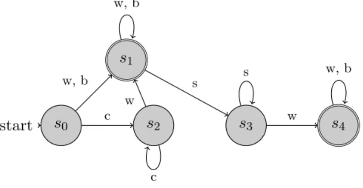
This state merging condition can be used to reduce the initial automaton presented in Figure 1. After the reduction is also antisymmetric and defines a partial order on the set of states. In this figure, statess1 and s3 verify the above-described condition and we can build the reduced automaton of Figure 3.
s0 start
s1
s2 s3 s4
w, b c
w, b
s
c w
w
s w, b
Figure 3: Reduced NFA for mode setM3 ={w, b, c, s}
Such a reduction is beneficial for the computational requirements as the previous sec- tion and computational experiments show that the complexity of the algorithms depends on the number of states of the NFA. We now propose the following state-based dominance rule.
Theorem 5.2 (State-based dominance rule). Consider two labels (i, s, k) and (i, s′, k′) withk≤k′,ss′ andtkis ≤tkis′′. Label(i, s, k)dominates(i, s′, k′), which can be discarded.
Proof. From the definition of relation , we know that any transition from s′ yields the same state as any transition from s. So label (i, s, k) has at least the same extension possibilities as label (i, s′, k′). The remaining conditions (k≤k′ and tkis ≤tkis′′) show that any extension of (i, s′, k′) is dominated by an extension of (i, s, k).
In the reduced automaton for mode setM3 ={w, b, c, s}(Figure 3), we see thats1s4 is the only dominance relation. The automaton for mode setM2={w, b, s}of Figure 2(b) cannot be reduced and dominance relations0 s2 holds.
Note that if transitions are represented by a matrix, all dominance relations can be established during preprocessing inO(|M|2|S|2) time.
In the algorithms described in the subsequent sections, different definitions of set Ds
can be used to parametrize the use of dominance rules:
• Ds=∅corresponds to no dominance checking (except the Bellman condition).
• Ds={s}corresponds to basic dominance checking.
• Ds={s′∈S|s′ s}corresponds to state-based dominance checking.
5.3 Topological label-setting (TLS) algorithm 5.3.1 Description
The topological Pallottino and Scutell`a [23] algorithm was extended by Lozano and Storchi algorithm [15] to path viability modeled by a NFA. We describe below a label-setting variant named TLS (the original algorithm of [15] being described as a label-correcting algorithm) with additional improvements and corrections.
This algorithm (pseudo-code is given in Algorithm 1 of Appendix A) iterates on the number of transfers from 0 tokmax. At each iterationk, it searches for the shortest path with exactlyk transfers. For that, the data structureQ for storing labels, is made of two priority queues Qnow and Qnext, where Qnow contains labels with k transfers and Qnext contains labels with k+ 1 transfers. Initially, Qnow contains only label (O, s0,0) while Qnext is empty.
At a typical iteration, the minimum time label (i, s, k) is taken fromQnowand the label extension principle (see Algorithm 2 of Appendix A) is applied with some modifications regarding the general label setting algorithm. To check the dominance rules, a variable, denoted byBestV aluej,s′, stores all algong the search the shortest travel time found so far to reach nodej in states′ (i.e. with at mostk transfers). The variable is used to have an O(1) basic dominance checking (instead of enumerating all tkjs′′′ such thatk′′< k′.) and a O(|Ds′|) state-based dominance checking (see Section 5.3.2). If the dominance condition holds, the label is discarded. Otherwise, if k = k′, BestV aluej,s′ is updated and the new label (j, s′, k′) is inserted inQnow. If k′=k+ 1; the label is inserted in Qnext.
Back to the TLS main procedure (Algorithm 1), as soon as the destination D is de- queued from Qnow or ifQnow becomes empty,Qnow is set toQnext and Qnext is emptied.
The algorithm stops whenQnextis empty, meaning that no nondominated labels withk+1 transfers could be found, or when the maximum number of transferskmax is reached.
To summarize, this version of TLS algorithm presents some improvments to the Lozano and Storchi algorithm [15]:
• A label-setting algorithm is proposed in place a label-correcting algorithm, following the recommendations of [26].
• At each iteration, when travel time of a new label is computed, the best travel time of previous solutions, denoted byBestLastSolis also used to prune labels (in addition toBestV alue).
• In [15], a single labeltis is used per node-state pair (i, s) for both extensions inQnow withktransfers and inQnext withk+ 1 transfers. However, a path with ktransfers may not be extended because it has a longer time than a path withk+ 1 transfers.
We correct this problem by defining two labels tkis and tk+1iq .
• We use the state-based dominance rule proposed in Section 5.2 instead of the one proposed in [15] (see Section 5.2 for justifications).
With TLS algorithm, solutions are obtained with increasing number of transfers and de- creasing travel times. In appendix B, the algorithm is applied to the instance described in Figure 2 with the state-based dominance rule. 12 labels are marked and 18 labels are reached.
5.3.2 Complexity
Complexity of dominance rule checks.
The basic dominance rule on label (j, s′, k′) can be performed in O(1). Indeed, for a given label (j, s′, k′), we have only to keep track of the shortest time found so far to reach (j, s′, k′′) with k′′ ≤ k′, denoted BestV aluejs′. A label (j, s′, k′) is dominated if tkjs′′ ≥BestV aluejs′, as the previously encountered label cannot have more transfers.
The complexity of the state-based dominance rule is in O(|S|): a given label (j, s′, k′) obtain by extension of a label (i, s, k) is dominated if BestV aluej,s′′ > tkis+dij for all states s′′ such thats′′s′.
Complexity of TLSWe now establish the complexity of our implementation of TLS using binary heaps forQnow and Qnext. Let kmax denotes the maximum allowed number of transfers. Notekmax is bounded from above by n|S|. For a given number of transfers k, at mostn|S|labels (i, s, k) are selected as minimum time labels in Qnow.
For each of them, there are two operations: (a) deletion from Qnow and (b) successor scan and insertion in Qnow or Qnext. Deletion from the binary heap can be done in O(log(n|S|)). Successor scan with the basic dominance rule (inO(1)) and possible insertion (inO(log(n|S|)) has a worst-case complexity inO(|F Si|log(n|S|)) whereF Si is the set of direct successors ofi. The complexity of operation (a) is ignored (neglected) since it is lower than the complexity of operation (b). It follows that the worst-case time complexity of TLS with the basic dominance rule and binary heap implementation isO(kmax|S||E|log(n|S|)).
Running the state-based dominance rule takes in addition|S|operations for each successor so we obtain in this case a worst-case complexity ofO(kmax|S||E|(|S|+ log(n|S|))).
5.4 Multi-queue label-setting (MQLS) algorithm 5.4.1 Description
We propose an alternative algorithm that computes the shortest paths in increasing order of the time criterion values and in decreasing order of the number of transfers. Instead of considering two queues Qnow and Qnext, we build incrementally a list Q ={Q0, Q1, . . .} of buckets (priority queues) such that each bucket Qk ∈ Q contains labels representing paths withk transfers. More precisely,Q0 is initialized with label (O, s0,0), all otherQk being empty. The number of bucketsK is set tokmax. At each iteration, the label (i, s, k) with minimum travel time is taken among all non-empty priority queues. If a destination label (D, s, k∗) is dequeued, priority queuesQk′ withk′ > k∗ are discarded andK is set to k∗−1, as the shortest path withk∗transfers toDis found. Otherwise, nondominated labels (j, s′, k′) such thatk′ ≤K issued from (i, s, k) are inserted in the corresponding priority queue Qk′ by the label extension procedure. The algorithm stops when the shortest path with 0 transfer is found or when all queues are empty. The algorithm pseudo code is given in Algorithm 3 of Appendix A. The Label Extension subroutine is given in Algorithm 4 of Appendix A. In appendix B, the algorithm is also applied to the instance described in Figure 2. 12 labels are marked and 16 labels are reached by the search.
We show the equivalence of TLS and MQLS in the sense they both have the nice feature described by the following property. As in the standard Dijkstra algorithm, a label is “marked” as soon as it is dequeued fromQ.
Proposition 5.3. The set of labels (i, s, k) marked by TLS or MQLS for a given (i, s) maps the set of all nondominated points for the bi-objectiveO−iviable path problem with
sas final state.
In particular, settingi=Dands∈F, we see that TLS and MQLS generates one and only one path for each nondominated point.
5.4.2 Complexity
We determine the algorithm complexity, using binary heaps for each Qk ∈ Q. In Q at mostkmaxn|S|labels are stored and dequeued (marked). For each iteration, there are three operations: (a) search of the minimum time value in thekmax queues; (b) deletion of the corresponding label inO(log(n|S|)); and (c) for each scanned successor, a dominance check is possibly followed by an insertion operation in the appropriate queue in O(log(n|S|)).
The basic dominance check can be made here in at most kmax operations as all labels (j, s′, k′′) with k′′ ≤k′ must be checked. So, with this dominance rule, the operation (c) has anO(|F Si|(kmax+ log(n|S|)) worst-case time complexity. The state-based dominance rule can be applied inO(kmax|S|), then the operation (c) as a worst-case time complexity ofO(|F Si|(kmax|S|+ log(n|S|)).
Taking account of (a) and (b) operations, with the basic dominance rule, we obtain a worst-case complexity of
O(kmax|S|(nkmax+nlog(n|S|) +|E|kmax+|E|log(n|S|)) =O(kmax|S||E|(kmax+ log(n|S|)). and, with the state-based dominance rule, this worst-case complexity is
O(kmax|S|(nkmax+nlog(n|S|) +|E|kmax|S|+|E|log(n|S|)) =O(kmax|S||E|(kmax|S|+ log(n|S|)). The worst-case time complexity is increased compared to the TLS algorithm by akmax
factor.
5.5 Bidirectional Multi-Queue Label Setting Algorithm (FB-MQLS) We propose a bidirectional adaptation of MQLS, taking advantage of the multi-queue characteristics. There are two main issues in designing a bidirectional algorithm for the considered multimodal problem. The first issue consists in modeling backward path via- bility. The second issue lies in exploiting the connection between a forward and backward label in the bi-objective context. The multi-queue structure will be here fully exploited as several label queues will be discarded when a given connection condition is reached.
These issues are addressed in Section 5.5.1 and the algorithm FB-MQLS is described in Section 5.5.2.
5.5.1 General Principles
The proposed bidirectional algorithm (FB-MQLS) maintains, in a similar way as in MQLS algorithm, two priority queue lists FQ for the forward search and BQ for the backward search such that F Qk contains forward labels f tki,s representing paths reaching i in state swith k transfers andBQk contains backward labelsbtki,s representing paths originating fromi withktransfers in state s.
Modeling backward path viability
We exhibit below three different possibilities to model backward path viability. Let
F A= (SF, M, δF, sF0, FF) denotes the automaton for the forward search and BA = (SB, M, δB, sB0, FB) the automaton for the backward search. To obtain BAfrom F A, the first possibility is simply to reverse the arcs of F A as done in [22]. In our case, for mode set M3, although the forward automaton is a DFA, the obtained state automaton be- comes non-deterministic (see left part of Figure 4). In this figure, the initial state (at destination) is sD. Final states are s1 (departure by walk or bus) and s2 (departure by private car). Transition functionδB(mi, mj, s) gives a set of possible states. For example δB(mD, w, sD) = {s1, s4} (where mD denotes the mode at the destination). This means what when arriving by walk at the destination, it could be that the subway was taken (states4) or was not taken (states1). In practice, each time a label extension uses an arc that yields several possible successor states (in the backward path), all the corresponding labels are generated. Note that such an indeterminism may yield pairs (i, s) that may never reach the origin, inducing useless computations.
The second possibility is to use a deterministic finite state automaton for the backward search. This is always possible as there exist algorithms that transform a non-deterministic finite state automaton equivalent to any deterministic one, however it can be that for a given non-deterministic automaton with|S|states, the equivalent deterministic automaton has less than 2|S| states. An issue then is to generate the deterministic automaton with a minimal number of states. Note that this issue also applies to the forward automaton which can be non-deterministic if it is obtained from a regular expression.
A third possibility is to obtain a (ǫ-free) NFA through the reverse regular expression, which can be done in polynomial time [24]. For example, the forward regular expres- sion corresponds to c*(w, b)*s*(w, b)* and the reverse regular expression corresponds to (w, b)*s*(w, b)*c*.
Comparing the different ways of obtaining the backward NFA for general forward NFA would be an interesting follow-up to the present study. In particular the speed-up obtained by optimizing the NFAs would have to be balanced with the CPU time needed to perform the NFA reductions and/or conversion to a minimum-state DFA. Nevertheless, to illustrate the potential gain of optimizing the (backward) NFA, we display, in right part of Figure 4, a possible deterministic finite state automaton forBAthat can we have obtained manually from the reverse regular expression.
The state-based dominance rule applies also for the backward automaton. For the non- deterministic automaton of Figure 4(b), there is no dominance relation between states in the sense of Theorem 5.2. For the deterministic automaton of Figure 4(c), we have e1 e4. The set of states that dominate a given forward (backward) state s is denoted DF(s) (DB(s)), respectively.
Connection and queue discarding rule
The second issue for designing a bidirectional algorithm for the considered problem is linked to connection consequences between a forward label and a backward label in terms of number of transfers. In case the backward automaton is simply obtained by a reversal of the forward arcs, a forward label (if, kf, sf) connects to a backward label (ib, kb, sb) if if =ib andsf =sb since the backward NFA has the same states as the forward NFA.
In case the backward automaton has been reduced, a correspondence must be es- tablished between the forward and the backward states. Let CSBA→F A(s) (respectively CSF A→BA(s)) denote the set of F A (resp. BA) states compatible with a given state sof BA (resp. F A). A forward label (if, kf, sf) connects to a backward label (ib, kb, sb) if if =ib andsf ∈CSBA→F A(sb) or, equivalently,sb ∈CSF A→BA(sf).
With the deterministic backward automaton case of Figure 4(c) and the forward au-
s0 start
s1
s2 s3 s4
w, b c
w, b
s
c w
w
s w, b
(a) Forward DFA forM3
sD
start
s1 s2
s4 s3
w, b
w,b w, b
c
c
s
w,b s
w,b
(b) Backward NFA forM3
eD
start e1
e3
e2
e4
w, b
w, b s
c s
w,b
c
w,b w,b
(c) Backward DFA forM3
Figure 4: Automata for the backward search
tomaton of Figure 3,CSF A→BA(s1) ={e1, e4} CSF A→BA(s2) ={e2},CSF A→BA(s3) ={e3} and CSF A→BA(s4) ={e1}.
We show now that, even if we use the reversed forward automaton for backward search, additional state compatibilities can be automatically established between forward and backward states, so as to have earlier connections without using a manually optimized backward automaton. We first define formally state compatibility:
Definition 5.3. Forward state sfx and backward state sby are compatible if, for any mode m the concatenation of any m-terminated mode string accepted by sfx with any reversed m-terminated input string accepted by sby is a valid string.
We now establish the forward/backward compatibility theorem (sufficient condition).
Theorem 5.3 (Forward/backward state compatibility). Forward state sfx and backward state sby are compatible ifsfx sfy in the forward automaton or ifsby sbx in the backward automaton.
Proof. If one of the dominance relation holds, the concatenation of any m-terminated mode string accepted by sfx with any reversed m-terminated input string accepted by sby is a valid string, yielding the desired compatibility.
In our example, there are no state-based dominance in the backward automaton but dominancesf1 sf4 holds in the forward one. Hence, since any input string accepted bysf4
is accepted bysf1, it follows that sb1 and sf4 are compatible states, on which a connection can be established.
Note that if dominance relations are represented by a |S| × |S| boolean matrix, all compatibility relations can be precomputed inO(|S|2) time.
In case of a connection, the interest of the multi-queue implementation appears. In- deed, when a connection is made between a label (if, h, sf) and a label (ib, q, sb) such that the statesf of F Ais compatible with state sb of BAand
f thi,sf +btqi,sb≤ min
(i′,s′,k′)∈FQf tki′′,s′ + min
(i′,s′,k′)∈BQbtki′′,s′
holds, all priority queuesF Qk′ andBQk′ withk′ ≥h+q can be discarded since the right hand side is a lower bound of the shortest path with at leasth+q transfers
5.5.2 Algorithm description
Algorithm FB-MQLS pseudo-code is given in Appendix A (Algorithm 5). FQis initalized to a single priority queueF Q0 with a single label (O, s0,0) andBQis initialized to a single priority queueBQ0 with a labels (D, sD,0). The upper bound of the number of transfers K is set to kmax. BestCurrentSolk stores the best known solution with k transfers and k∗ corresponds to the number of transfers of the current best known solution.
The main loop computes the minimum time forward label (if, sf, kf) and the minimum time backward label (ib, sb, kb). The search proceeds from the minimum time label among them, denoted by (i, s, k). The minimum time label (i, s, k) is then removed from its priority queue (F Qk or BQk) and the forward or backward label extension principle is performed in a similar way as the MQLS Label extension.
The main difference is that (for instance in the forward extension), for each new non- dominated label (j, s′, k′), a connection with the opposite direction search is searched by scanning all labels (j, sb, k′′) withk′+k′′≤K andsb∈CSF A→BA(s′) which possibly yields anO−Dpath of less than K transfers. If such a connection is established, its path time (f tkj,s′′+btkj,s′′b) is compared against the bestO−Dpath already found withk′+k′′transfers whose time is stored as BestCurrentSolk′+k′′, to possibly update it. Moreover, if the given forward label (j, s′, k′) is connected with a marked-up backward label with 0 transfer then label (j, s′, k′) can be discarded as all nondominated shortest paths fromDtoihave been found. The forward label extension algorithm is given in Algorithm 6. The backward label extension algorithm is symmetrical and not given in the paper.
After the forward or backward label extension, the queue discarding rule compares the minimum timeBestCurrentSolk∗ obtained among already established connections, with the lower bound given by the sum of the minimum forward and backward label times (f tkiff,sf +btkibb,sb). If the test is affirmative, BestCurrentSolk∗ is the best path time for k∗ transfers and priority queuesF Q˜k and BQ˜k with ˜k≥k∗ can be discarded.
We show in Apendix B the execution of this algorithm for the example of Figure 2.
The algorithms marks 8 labels and reaches 22 labels.
5.5.3 Complexity
Compared to MQLS, there is a computational overhead (only at label extension) induced by connection search (step 14 of Algorithm 6). Let us examine first this overhead in terms of complexity for the forward extension. With the basic dominance rule, recall