Fluid-structure interaction using a partitioned semi-implicit predictor-corrector coupling scheme for the application of large-eddy simulation

HAL Id: hal-01018330

https://hal.archives-ouvertes.fr/hal-01018330

Submitted on 4 Jul 2014

HAL is a multi-disciplinary open access archive for the deposit and dissemination of sci- entific research documents, whether they are pub- lished or not. The documents may come from teaching and research institutions in France or abroad, or from public or private research centers.

L’archive ouverte pluridisciplinaire HAL, est destinée au dépôt et à la diffusion de documents scientifiques de niveau recherche, publiés ou non, émanant des établissements d’enseignement et de recherche français ou étrangers, des laboratoires publics ou privés.

Distributed under a Creative CommonsAttribution - NonCommercial - NoDerivatives| 4.0 International License

semi-implicit predictor-corrector coupling scheme for the application of large-eddy simulation

Michael Breuer, Guillaume de Nayer, Manuel Münsch, Thomas Gallinger, Roland Wüchner

To cite this version:

Michael Breuer, Guillaume de Nayer, Manuel Münsch, Thomas Gallinger, Roland Wüchner. Fluid- structure interaction using a partitioned semi-implicit predictor-corrector coupling scheme for the application of large-eddy simulation. Journal of Fluids and Structures, Elsevier, 2012, 29, pp.107-130.

�10.1016/j.jfluidstructs.2011.09.003�. �hal-01018330�

predictor–corrector coupling scheme for the application of large–eddy simulation

M. Breuer^a,∗, G. De Nayer^a, M. M¨unsch^b, T. Gallinger^c, R. W¨uchner^c

aProfessur f¨ur Str¨omungsmechanik, Helmut–Schmidt–Universit¨at Hamburg, D–22043 Hamburg, Germany

bLehrstuhl f¨ur Str¨omungsmechanik, Universit¨at Erlangen–N¨urnberg, D–91058 Erlangen, Germany

cLehrstuhl f¨ur Statik, Technische Universit¨at M¨unchen, D–80290 M¨unchen, Germany

Abstract

The paper is concerned with an efficient partitioned coupling scheme developed for dynamic fluid–structure interaction problems in turbulent flows predicted by eddy–resolving schemes such as large–eddy simulation (LES). To account for the added–mass effect for high density ratios of the fluid to the structure, the semi–implicit scheme guarantees strong coupling among flow and structure, but also maintains the advantageous properties of explicit time–marching schemes often used for turbulence simulations. Thus by coupling an advanced LES code for the turbulent fluid flow with a code especially suited for the prediction of shells and membranes, an appropriate tool for the time–resolved prediction of instantaneous turbulent flows around light, thin–walled structures results. Based on an established benchmark case in laminar flow, i.e., the flow around a cylinder with an attached flexible structure at the backside, the entire methodology is analyzed thoroughly including a grid independence study. After this validation, the benchmark case is finally extended to the turbulent flow regime and predicted as a coupled FSI problem applying the newly developed scheme based on a predictor–corrector method.

The entire methodology is found to be stable and robust. The turbulent flow field around the flexible structure and the deflection of the structure itself are analyzed in detail.

Keywords: Fluid–structure interaction; partitioned scheme; large–eddy simulation; FSI benchmark; (artificial) added–mass effect; semi–implicit scheme

1. Introduction

Fluid–structure interaction is a topic of major interest in many fields such as mechanical engineering, civil engineering or medicine technique to mention only a few. Beside experimental investigations numerical simulations have become an important and valuable tool for solving this kind of problems. Two issues have led to a a great leap forward in the last years. On the one hand the numerical algorithms for the single fields experience substantial progress. On the other hand the available computational resources have strongly increased. Both developments now allow to tackle practically relevantdynamic fluid–structure interaction problems involving turbulent flow fields.

The long–term objective of the present investigation is to tackle civil engineering FSI applica- tions involving lightweight structures such as awnings, large umbrellas, and tent roofs, exposed

∗Corresponding author

Email address: breuer@hsu-hh.de(M. Breuer)

Preprint submitted to Elsevier July 4, 2011

to the turbulent wind field. Right from the start it was clear that highly advanced solvers for both subtasks are required for this purpose, i.e., a specialized (finite–element) solver for shells and membranes (Bletzinger et al., 2006; Fischer et al., 2010), and a specialized (finite–volume) solver relying on eddy–resolving methods such as large–eddy simulation (LES) (Breuer, 2002).

Thus monolithic coupling (see, e.g. Heil, 2004) is ruled out and apartitioned scheme is favored.

This idea goes back to the early work of Felippa and Park, (e.g., Park et al., 1977; Felippa and Park, 1980; Park, 1980; Park and Felippa, 1983; Felippa and Geers, 1988) named Staggered Solution Procedure. The strength of this approach originates from its modularity and the capa- bility of using for each sub-problem the most adapted method to its mathematical properties.

Examples of successful applications of this general concept are too numerous to be reviewed here. Furthermore, much work has been dedicated to the improvement of this concept (see, e.g., Piperno et al., 1995). Partitioned schemes are further classified into loosely and strongly coupled schemes. If the fluid dynamical problem and the structural problem are solved in a staggered manner without any subiterations, the coupling conditions at the interface are not exactly satisfied at each time step. The scheme is called loosely coupled and works in par- ticular in aeroelastic applications or in applications involving compressible viscous fluids (see, e.g., Farhat, 2004; Farhat et al., 2006). However, in many other cases weakly coupled schemes were found to be apparently unstable. Involving an incompressible viscous fluid and certain density ratios between the fluid and the structure, the so-called (artificial) added–mass effect may become an issue of major concern and strongly coupled schemes are essential (see, e.g., Causin et al., 2005; F¨orster et al., 2007; F¨orster, 2007) as in the current study. During the last years a variety of publications have been devoted to the development of efficient coupling algorithms for the non–linear FSI problem arising from the strongly coupled concept. Among these are the fixed–point iterations with fixed or dynamic underrelaxation (e.g., Mok, 2001;

K¨uttler and Wall, 2008; Degroote et al., 2008), vector extrapolation (e.g., K¨uttler and Wall, 2009) or Newton–based methods. For the latter recent overviews can be found in K¨uttler (2009), Gallinger (2010) and Vierendeels et al. (2010).

Fern´andez et al. (2007) suggested just another coupling concept which they call a partially explicit or semi–implicit scheme. Since that has a lot in common with the scheme proposed independently in Breuer and M¨unsch (2008, 2010) building the basis for the present paper, a brief overview should be provided. Applying the projection method developed by Chorin (1968) and Temam (1969a,b) for the solution of the incompressible fluid flow, this scheme is extended towards FSI problems. They proposed to strongly couple the projection sub-step carried out in a known fluid domain with the structure, while the ALE advection–diffusion sub-step is only weakly, i.e. explicitly, coupled to the structure. Hence the added–mass effect is accounted for in an implicit manner, but an implicit treatment of the ALE advection–diffusion sub-step known to be particularly expensive is avoided. Starting with the extrapolation of the fluid–structure interface (step 0), the new fluid domain is defined in step 1 followed by the explicit solution of the advection–diffusion problem (step 2). The projection step consisting of the solution of the pressure equation and the governing equation for the structure, are sub-iterated in step 3. In a rigorous theoretical evaluation the conditional stability of the scheme was proven for a linear model problem. Furthermore, the efficiency of the method compared to fully implicitly coupled schemes was shown in different numerical experiments on laminar flows using a finite–element discretization on both fields (Fern´andez et al., 2007).

In the present work we are interested in the simulation of turbulent flows including FSI. Direct numerical simulation and Reynolds–Averaged Navier–Stokes (RANS) equations with statistical turbulence models are not applicable either due to their enormous CPU–time requirements or their inability to predict non–equilibrium turbulent flows. Eddy–resolving schemes such as

large–eddy simulation (LES) or hybrid LES–RANS approaches as for example detached–eddy simulation (DES) have become popular for this purpose due to their favorable capabilities of predicting complex turbulent flows (Breuer, 2002). That is especially true for instantaneous flow processes involving large–scale flow structures such as separation, reattachment and vortex shedding. Flow phenomena of such kind are very often encountered when the flow around or through a device enforces the structures to be deformed or displaced, i.e. for fluid–structure interaction. Therefore, LES is also the preferential method in the context of FSI applications and therefore considered in the present study. However, LES is not well established in the FSI context up to now. In a recently published book on modeling and simulation for FSI (Bungartz et al., 2010) only two out of 15 contributions briefly touched the topic without going into details. At least three topics are of major concern to completely marry FSI and LES:

(i) The grid movement in ALE–FSI formulations generally means that also the filter width varies in time leading to additional commutation errors. This issue was addressed in Breuer and M¨unsch (2010) and M¨unsch and Breuer (2010).

(ii) For moving grids the question arises how the grid quality can be maintained during the instantaneous simulation. It is well-known that the demands on the grid quality regarding smoothness and orthogonality are higher for LES than for RANS. On the other hand the quality has to be assured at each time step requiring efficient and robust schemes. Beside using algebraic approaches also elliptic grid smoothing techniques (Spekreijse, 1995) have to be taken into account.

(iii) Furthermore, LES differs also with respect to the time resolution issue and thus adapted coupling schemes are favorable.

The present paper is intended to contribute especially to the last issue by proposing a FSI coupling method adjusted to the requirements of LES. The LES technique is based on spatial filtering of the instantaneous Navier–Stokes equations. The large scales are predicted directly by solving the filtered Navier–Stokes equations with a time–accurate scheme involving small time steps and modeling solely the small scales. For that purpose often predictor–corrector schemes are taken into account. Thus a methodology is suggested which relies on this specific time–marching scheme while taking into consideration that a strong coupling is needed to guarantee a stable and robust algorithm.

The paper is organized as follows. At first the numerical methodologies for both single fields are described separately in§2. In the subsequent section (§ 3) the coupling scheme developed is explained in detail. Then in § 4 a description of the test cases is provided explaining all details required to define the cases from the physical point of view. In§5 the specific numerical setups used in the present study are given. Finally, the results are presented in§6 split up into the validation procedure based on the laminar case and the final outcome for the turbulent case.

2. Numerical Methodology for Each Specific Field

2.1. Computational Fluid Dynamics (CFD) 2.1.1. Governing Equations

Within a FSI application the fluid forces acting on the structure lead to the displacement or deformation of the structure. Thus the computational domain is no longer fixed but changes in

time, which has to be taken into account. Besides other numerical techniques, the most popular one is the so-called Arbitrary Lagrangian–Eulerian (ALE) formulation. Here the conservation equations for mass and momentum, which are to be solved based on a finite–volume scheme, are re-formulated for a temporally varying domain, i.e., control volumes (CV) with time–

dependent volumesV(t) and surfacesS(t). Hence the governing equations in ALE formulation expressing the conservation of mass and momentum read:

d dt

Z

V(t)

ρ^fdV + Z

S(t)

ρ^f(uj −ug,j)·nj dS = 0, (1)

d dt

Z

V(t)

ρ^fui dV + Z

S(t)

ρ^fui(uj −ug,j)·nj dS = − Z

S(t)

(τij +τ_ij^SGS)·nj dS− Z

S(t)

p·ni dS .(2)

These are the (filtered) Navier–Stokes equations for an incompressible fluid assuming tempera- ture–independent fluid properties. Overbars typically used to denote filtered quantities within a large–eddy simulation are omitted here. Thus, the density of the fluid is denoted byρ^f, the pressure bypand the three Cartesian components of the velocity vector by ui. The molecular momentum transport tensor is indicated by τij whereas nj describes the unit normal vector pointing outwards. In case of LES, an additional tensor denoted τ_ij^SGS has to be taken into account in the surface integral on the right-hand side of eq. (2) describing the influence of the non–resolved subgrid–scales (SGS) on the resolved flow field (see § 2.1.2). Since the grid is deformable, the grid velocity with which the surface of a CV is moving is taken into account via ug,j. Here, the volume integrals now describe local changes in a CV of variable shape and thus the additional mass and momentum fluxes due toug,j. Since the system of equations given by (1) and (2) is not closed anymore, the unknown grid velocity u_g,j has to be determined. To compute this grid velocity while considering the conservation principle and avoiding the loss of mass and momentum, the so-called space conservation law (SCL)(Demirdˇzi´c and Peri´c, 1988, 1990) or geometric conservation law (GCL) (Lesoinne and Farhat, 1996) is applied:

d dt

Z

V(t)

dV − Z

S(t)

ug,j · njdS = 0 . (3)

This extra conservation law assures that within a change of the position or the shape of a CV no space is lost. In discretized form the SCL is expressed by the swept volumes of the corresponding cell faces. Inserting eq. (3) into (1), the mass conservation equation for a fixed grid is obtained:

Z

S(t)

uj ·nj dS = 0. (4)

Thus the prediction of extra grid fluxes is not necessary for the mass conservation equation in the context of moving grids. The additional grid fluxes in the momentum equation, however, have to be consistently determined by applying the SCL in its discrete form denoted discrete geometric conservation laws (DGCL) (Farhat et al., 2001). In the context of the Runge–

Kutta time–marching scheme (see§ 2.1.3) applied in the present study, a consistent numerical formulation reads

Z

S(t)

(ρ^fuiug,j) · njdS ≈ X

k={e,w,n,s,t,b}

µ ρ^fui,k

δV_kⁿ⁺¹

∆t

¶

, (5)

where the grid fluxes are split up into six contributions according to the six surfaces of the hexahedral CV, i.e.,east, west,north, south, top and bottom. Thereby the differences between the volumes of the CV between the new (superscript n + 1) and the old time step (n) can be expressed by the sum over the swept volumesδVkof all surfaces. In the three–dimensional case special care is required for the determination of the swept volumes since edges of CV surfaces can turn. Thus a segmentation into six tetrahedra possessing the same diagonal (Kordulla and Vinokur, 1983) is absolutely necessary in order to guarantee the correct prediction of the swept volumes.

2.1.2. Subgrid–Scale Modeling

In principle, the LES concept leads to a closure problem similar to that obtained by RANS.

However, the non–resolvable small scales in a LES are much less problem–dependent than the large–scale motion so that the subgrid–scale turbulence can be represented by relatively simple models, e.g., zero–equation eddy–viscosity models. Like other eddy–viscosity models the well- known and most often used Smagorinsky model (Smagorinsky, 1963) is based on Boussinesq’s approximation which describes the stress tensor τ_ij^SGS as the product of the strain rate tensor Sij1 and an eddy viscosity νT,

τ_ij^SGS,a = τ_ij^SGS−δij τ_kk^SGS/3 = −2νT Sij with Sij = 1 2

µ∂ui

∂xj

+ ∂uj

∂xi

¶

, (6)

where τ_ij^SGS,a is the anisotropic (traceless) part of the stress tensor τ_ij^SGS and δij is the Kro- necker delta. The trace of the stress tensor is added to the pressure resulting in the new pressure P =p+τ_kk^SGS/3. The eddy viscosity ν_T itself is a function of the strain rate tensor Sij and the subgrid length l, as

νT = l² |Sij | with l = Cs ∆

"

1 − exp

µ−y⁺ A⁺

¶3#0.5

,

∆ = (∆x·∆y·∆z)^1/3 , y⁺ = y uτ

ν , uτ = rτw

ρ^f and A⁺ = 25 . (7)

Here, τw,uτ and y⁺ denote the wall shear stress, the wall shear stress velocity and the dimen- sionless wall distance, respectively. The filter width ∆ is directly coupled to the volume of the computational cell. Cs is the well-known Smagorinsky constant which has to be prescribed as a fixed value or can be determined as a function of time and space by the dynamic procedure originally proposed by Germano et al. (1991) and later improved by several authors, e.g. Lilly (1992). In the first case, a Van Driest damping function as given in eq. (7) is required in order to take the reduction of the subgrid length l near solid walls into account. Owing to minor influences of SGS modeling at the moderate Reynolds number considered in this study, in the present investigations the fixed parameter version of the Smagorinsky model is applied using the well established standard constant Cs = 0.1.

As mentioned in the introduction, the grid movement in ALE–FSI formulations leads to addi- tional commutation errors due to the temporally varying filter width. In Breuer and M¨unsch (2010) and M¨unsch and Breuer (2010) this issue was addressed by investigating the influence of deforming grids on the quality of LES predictions. For this purpose, harmonic grid movements

1Overbars omitted as mentioned above.

with specific amplitudes and periods have been forced to a turbulent plane channel flow apply- ing the Smagorinsky model as well as the dynamic model. A variety of cases was considered.

In one subset of cases, the amplitude of the internal grid deformation was varied and the period of the deformations was fixed. In a second subset, computations for different cycle periods at a constant amplitude were performed. The results were compared to LES predictions on a fixed grid. Comparing both SGS models, the Smagorinsky model showed less deviations from the reference case than the dynamic model. Furthermore, the mean values were observed to be less sensitive than the second–order moments. As long as the amplitudes and frequencies of the oscillations were not too high, the impact on the flow properties was found to be minor.

Generally, hints on what kind of grid motions are tolerable within an FSI application using LES were obtained.

2.1.3. Discretization Spatial Discretization.

For the present study the in-house code FASTEST-3D (Durst and Sch¨afer, 1996; Durst et al., 1996) is used and extended for the FSI–LES application intended. The code is based on a three–

dimensional finite–volume scheme which is used to discretize the governing equations (1) to (5) in ALE formulation. The discretization is done on a curvilinear, block–structured body–

fitted grid with colocated variable arrangement by applying standard schemes. A midpoint rule approximation of second–order accuracy is used for the discretization of the surface and volume integrals. Furthermore, the flow variables are linearly interpolated to the cell faces leading to a second–order accurate central scheme. In order to ensure the coupling of pressure and velocity fields on non–staggered grids, the momentum interpolation technique of Rhie and Chow (1983) is used.

Temporal Discretization.

For LES small time steps are required to resolve the turbulent flow field in time which leads to a preferred usage of explicit time–marching schemes. Here, a predictor–corrector scheme of second–order accuracy forms the kernel of the fluid solver. In the predictor step an explicit three substep low–storage Runge–Kutta scheme advances the momentum equation in time leading to a prediction of the velocities u^∗_i. These predicted velocities do not satisfy mass conservation. Thus, in the following corrector step the mass conservation equation has to be fulfilled by solving a Poisson equation for the pressure–correction based on the incomplete LU decomposition method of Stone (1968). The corrector step is repeated until a predefined convergence criterion is reached and the final velocities and the pressure of the new time step are obtained. Hence the predictor–corrector step is also a projection method as originally proposed by Chorin (1968) and Temam (1969a,b). The procedure described was developed for fixed grids. Thus the question arises how to extend this predictor–corrector scheme to moving or deforming grids. However, inserting eq. (3) into (1) the mass conservation equation for a fixed grid is obtained. Therefore, the original pressure–correction scheme applied for the solution of the incompressible Navier–Stokes equations on fixed grids has not to be changed concerning the mass conservation equation in the context of moving grids. Solely in the momentum equation the grid fluxes have to be taken into account as described above. For achieving mass conservation the pressure–correction algorithm is repeated until a predefined convergence criterion ε is reached leading to the final velocities ui and the corresponding pressure field p of the new time step. For the present algorithm and test cases, typically 3 to 8 pressure–

correction iterations are required until the mass conservation equation is numerically satisfied, e.g. ∆ ˙m < ε=O(10⁻⁹).

FASTEST-3D is highly vectorized and additionally parallelized by domain decomposition with explicit message–passing based on MPI allowing efficient computations on vector–parallel ma- chines and SMP clusters.

2.1.4. Grid Adaptation

As will be shown below, the coupling between fluid and structure takes place at the interface between both domains. From the viewpoint of the CFD prediction, forces on the structure have to be provided for the CSD calculation and even of stronger impact displacements at the boundaries of the computational domain for the fluid flow are delivered by CSD. As a conse- quence the task is to adapt the grid of the inner computational domain based on displacements provided solely at specific boundaries, i.e., the interface with the structure. The choice of an appropriate method is subject of the following constraints: The grid adaptation has typically to be done several times during each time step. Therefore, fast and efficient methods are of great importance. On the other hand, to maintain the grid quality, i.e., orthogonality and smoothness, and according to these properties the accuracy of the numerical prediction for time–dependent and moving grids, is a mandatory issue for FSI algorithms, especially for tur- bulent flows using the LES approach. For moderate deformations algebraic methods are found to be a good compromise since they are extremely fast and deliver reasonable grid point dis- tributions. Another issue for the choice of the appropriate method is the question whether the algorithm can be fully parallelized, which is the case for algebraic methods. Thus, considering all arguments, the grid adjustment is presently performed based on a transfinite interpolation (Thompson et al., 1985). It consists of three shear transformations plus a tensor–product trans- formation. Beside using this algebraic approach also developments on elliptic grid smoothing based on a composite mapping (Spekreijse, 1995) consisting of a non–linear transfinite alge- braic transformation and an elliptic transformation are currently under development for strong grid deformations.

2.2. Computational Structural Dynamics (CSD) 2.2.1. Governing Equations

Based on the continuum mechanics assumption the dynamic equilibrium of the structure is described by the momentum equation given in a Lagrangian frame of reference. Allowing large deformations, where geometrical non–linearities are not negligible, the following boundary value problem has to be considered (Hojjat et al., 2010):

ρ^s ∂²d

∂t² = ∇ ·(F · S) + ρ^sb. (8)

Hereρ^s denotes the density of the structure,dthe displacement of the material point in space, F the material deformation gradient, S the second Piola–Kirchhoff stress tensor and b the specific volume forces. A constitutive relation providing a link between stress and strain is required to close eq. (8). For a St. Venant–Kirchhoff material with C being the constitutive tensor andErepresenting the Green–Lagrange strain, the second Piola–Kirchhoff stress tensor is given by

S = C : E, E = 1

2(F^T ·F − I) (9)

2.2.2. Discretization

For the solution of the governing equation (8) for the structure, i.e. the computational structural dynamics (CSD), the finite–element solver Carat++ (Fischer et al., 2010; Bletzinger et al.,

2006) developed by TU Munich especially for the prediction of shell or membrane behavior is applied. Carat++ is based on several finite–element types and advanced solution strategies for form finding and non–linear dynamic problems. For the dynamic analysis, different time–

integration schemes are available, e.g. the implicit generalized–α method (Chung and Hulbert, 1993). In the modeling of thin–walled structures, membrane or shell elements are applied for the discretization within the finite–element model. In the current case, the plate is modeled with a seven–parameter shell element. Furthermore, special care is given to prevent locking phenomena by applying the well-known ANS and EAS methods (Bischoff et al., 2004).

Both, shell and membrane elements reflect geometrically reduced structural models with a two–dimensional representation of the mid–surface which can describe the three–dimensional physical properties by introducing mechanical assumptions for the thickness direction. Due to this reduced model additional operations are required in the structural part to transfer information between the two–dimensional structure and the three–dimensional fluid model.

Thus in the case of shells, the surface of the interface is found by moving the two–dimensional surface of the structure half of the thickness normal to the surface on both sides and the closing of the volume (Bletzinger et al., 2006). On these two moved surfaces the exchange of data (see

§ 3) is performed consistently with respect to the shell theory (Hojjat et al., 2010).

3. Coupling Algorithm

3.1. Preliminary Considerations

The choice of the coupling scheme suggested is motivated by the following considerations and constraints:

• Both the CSD code Carat++ and the CFD code FASTEST-3D are highly adapted to their specific field of application, providing many special features. To preserve these ad- vantages and to realize an effective coupling algorithm, a partitioned solution approach is chosen. In comparison to the monolithic approach based on a unified numerical for- mulation of the whole FSI problem, the partitioned one possesses a stronger universality and allows to exchange codes for each subtask if appropriate.

• The method of choice for the prediction of instantaneous non–equilibrium flow processes involving large–scale flow structures (separation, reattachment, vortex shedding) very often encountered in FSI problems, is the LES technique. In contrast to the RANS approach which is not an appropriate choice for such kind of flows, LES typically requires small time steps to resolve the turbulent flow field in time which leads to a preferred usage of explicit time–marching schemes. Here, a predictor–corrector scheme of second–order accuracy forms the kernel of the fluid solver (see §2.1.3). Thus the coupling scheme has to rely onexplicit predictor–corrector schemes.

• For the partitioned coupling between the fluid solver and the structure solver in general two different methodologies can be distinguished. Within the so-called loose coupling approach the fluid and the structure subproblem are only solved once per time step leading to severe stability problems in many applications. Thus the strong coupling approach accounting for the (strong) added–mass effect (see, e.g., Causin et al., 2005;

F¨orster et al., 2007; F¨orster, 2007) is favored here, where the solution of both subproblems are repeated in a staggered manner until a dynamic equilibrium is achieved.

The task is to marry FSI and LES by considering all relevant aspects mentioned. Thus aparti- tioned butstrong coupling scheme relying on aexplicit predictor–corrector scheme is requested meeting the requirements for an efficient large–eddy simulation on the one hand and a stable coupling algorithm on the other hand.

3.2. Coupling Scheme

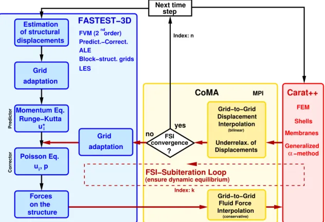
In § 2.1.3 the original predictor–corrector scheme for the fluid flow is explained. For coupled FSI computations this basic algorithm is extended as depicted in Fig. 1 and suggested in a similar manner already in Fern´andez et al. (2007). Based on the velocity and pressure field from the corrector step, the fluid forces resulting from the pressure and the viscous shear stresses at the interface between the fluid and the structure are computed. These forces are transferred to the CSD code Carat++ using the conservative interpolation scheme described in§ 3.3 and implemented in CoMA.

Using the fluid forces provided via CoMA, the finite–element code Carat++ determines the stresses in the structure and the resulting displacementsd_newof the structure. This response of the structure is transferred back to the fluid solver via CoMA applying a bilinear interpolation also given in§ 3.3.

Forces on the Estimation of structural displacements

Momentum Eq.

Runge−Kutta

Poisson Eq.

structure

step

Grid

Next time

? u*

u , p

PredictorCorrector

Block−struct. grids ALE

Predict.−Correct.

nd

i i

adaptation

FSI convergence

yes no

LES

FSI−Subiteration Loop

(conservative)

FASTEST−3D

FVM (2 order)

CoMA ^MPI

Interpolation Grid−to−Grid Fluid Force Grid−to−Grid

(ensure dynamic equilibrium)

Displacement Interpolation

(bilinear)

Displacements Underrelax. of

Carat++

FEM

Generalized α_−method Membranes Shells Index: n

Index: k

Grid adaptation

Figure 1: Sketch of the partitioned strong FSI coupling scheme including the FSI–subiteration loop.

In the case of a loose coupling approach the displacements are considered to be the physically correct displacements of the actual time step. With respect to the flowchart in Fig. 1, it means that FSI convergence is assumed to be achieved. Thus the computation would pass on to the successive time step. However, this loose coupling between fluid and structure is in general

only stable for low density ratios of the fluid to the structureρ^f/ρ^s ¿1, i.e., in case of a low so-called added mass effect (Causin et al., 2005; F¨orster et al., 2007; F¨orster, 2007).

A typical application for this situation is encountered in aeroelasticity (Farhat, 2004), i.e., a wing of high structural density ρs exposed to a fluid flow of air possessing a low fluid density ρf. Consequently, a low density ratio ρ^f/ρ^s results. If the wing oscillates up and down, the structure has to also accelerate the fluid around the deformed or oscillating wing. That leads to additional fluid forces acting on the surface in contact with the fluid denoted as added–mass effect. Owing to the low density ratio of the air to the structure, the structure hardly senses the fluid. Thus its added mass is of minor importance and a loose coupling scheme is reasonably (Farhat, 2004; Farhat et al., 2006).

For cases of moderate and high density ratiosρ^f/ρ^s, e.g., a flexible structure exposed to a fluid flow of e.g. water, the structure strongly feels the surrounding fluid. Then the added–mass effect by the surrounding fluid plays a dominant role. In such situations loose coupling schemes typically tend to fail, especially in the context of incompressible flows. Thus a strong coupling scheme as suggested in the present study taking the tight interaction between the fluid and the structure into account, is indispensable. For that purpose a so-called FSI–subiteration loop is established in the coupling scheme developed (see Fig. 1) which works in the following manner:

• Convergence check:

First the FSI convergence is checked. For that purpose it has to be inspected whether the dynamic equilibrium between fluid and structure is numerically achieved. The crite- rion can either rely on the displacements of the structure or the loads on the interface.

Presently, the change of the resulting displacements within the FSI–subiteration cycle are taken into account. Convergence is reached if the L₂ norm of these displacement differences between two FSI–subiterations (index k) normalized by the L2 norm of the changes in the displacements between the current and the last time step (index n), i.e.,

||d^n,k − d^n,k−1||2

||d^n,k − dⁿ⁻¹ ||2

< εF SI (10)

drops below a predefined limit, e.g. εF SI = 10⁻⁵ for the test cases of the present study.

• Grid adaptation:

Typically, convergence is not reached within the first step. Therefore, the procedure has to be continued on the fluid side. Based on the displacements on the fluid–structure interface, the inner computational CFD grid is adjusted as described in §2.1.4.

• Core of the coupling scheme / Repetition of corrector step:

Subsequent to the grid adaptation solely the corrector step of the predictor–corrector scheme is performed again and a new velocity and pressure field is obtained. Since this issue is the key point of the coupling procedure suggested, some more explanations should be added.

In contrast to the present coupling scheme relying on explicit time marching, within a coupling scheme based on fully implicit time stepping as used, e.g., in Gl¨uck et al.

(2001, 2003), an inner CFD loop becomes necessary within the applied SIMPLE scheme (Patankar and Spalding, 1972). Consequently, both schemes significantly differ with respect to the momentum equations within the FSI–subiteration loop. For the implicit scheme the momentum equations are solved repeatedly in each subiteration sweep. In contrast they are only solved once per time step for the explicit case which strongly

reduces the computational effort. Furthermore, the number of FSI–subiterations required to reach the convergence criterion is typically much smaller for the explicit scheme (Breuer and M¨unsch, 2008, 2010; M¨unsch and Breuer, 2010) than for the implicit variant (Gl¨uck et al., 2001, 2003).

The clue is the pressure, which is the most important quantity when solving incompress- ible fluid flow problems. The predictor–corrector scheme guarantees that the pressure is determined in such a manner that the velocity field is finally divergence–free and mass conservation is satisfied. Furthermore, the extension of the predictor–corrector scheme towards the FSI–subiteration loops assures that the most relevant forces for the added–

mass effect, i.e. the pressure forces, are successively updated until dynamic equilibrium is achieved. In conclusion, instabilities due to the added–mass effect known from loose coupling schemes are strongly reduced or completely avoided by the newly developed coupling scheme and the explicit character of the time–stepping scheme beneficial for LES is still maintained.

To concretize the comparison of both algorithms, in Gl¨uck et al. (2001) a typical number of about 1000 CFD iterations is provided for an average time step of the fully implicit scheme. That means that at each time step all three non–linear momentum equations as well as the pressure correction equation have to be solved thousand times, e.g. 4000 equations. For the present scheme, the coupling scheme is found to require only a few FSI–subiterations (5 to 10, average about 7.5) to go below the convergence limit ensuring dynamic equilibrium. As mentioned above, within each subiteration 3 to 8 (average about 5.5) pressure–correction iterations are necessary leading in average to 7.5× 5.5 ≈ 41 required solutions per time step. Together with the solution of the momentum equations a ratio of about 44 / 1000 ≈ 1 / 23 is obtained providing at least a rough estimation about the computational effort per time step required for both schemes. Thus especially for small time steps (used in LES), the scheme developed works very efficiently.

• Closure of the FSI–subiteration loop:

After a new pressure and velocity field is available, new loads for the structure solver are determined. Again these are transferred via CoMA to Carat++ leading to an update of the corresponding displacements by solving the equations of non–linear elastodynamics.

The displacements are sent back via CoMA to FASTEST-3D closing the FSI–subiteration loop (see Fig. 1).

• Initializing a new time step / Estimation of displacements:

Based on the convergence criterion mentioned above, it is decided whether the subiter- ation process is continued or stopped. In the latter case the computation for the next time step is started. The new time step begins with an estimation of the displacement

˜d of the structure. In contrast to the strong coupling scheme relying on a fully implicit time–marching algorithm (Gl¨uck et al., 2001, 2003), in the present scheme this measure does not only serve for convergence acceleration within the coupling process but also ensures that the momentum equations are solved on the updated geometry, which is an important feature. For the estimation two versions are taken into account. Either a first–

order linear or a second–order parabolic extrapolation is applied for the displacements by taking the displacement values of two or three former time steps indicated by the superscripts ⁿ⁻¹,ⁿ⁻², and ⁿ⁻³ into account:

linear: ˜dⁿ = 2dⁿ⁻¹ − 1dⁿ⁻² , (11)

parabolic: ˜dⁿ = 3dⁿ⁻¹ − 3dⁿ⁻² + 1dⁿ⁻³ . (12)

Tests with the parabolic second–order extrapolation (12) have shown no improvements of the results and no better convergence than for the linear version (11). An explanation for this behavior is given by the small time–step size of the explicit time–stepping scheme.

According to these estimated boundary values, the entire computational grid has to be adapted as it is done in each FSI–subiteration loop. Once the grid is adapted, the predictor–corrector scheme of the next time step is carried out and the cycle of the FSI–subiteration loop is entered again.

Significant structural deformations can be taken into account by an underrelaxation of the boundary geometry. The grid adaptation is then based on an underrelaxation of the structural response d^k_new by taking an underrelaxation factor ω and the displacement of the previous subiteration loop (k−1) into account:

d^k_new = ωd^k + (1 − ω)d^k−1 , (13) wherek denotes the subiteration counter. The underrelaxation factorωcan either be assumed to be constant or dynamically predicted based on the Aitken method (Aitken, 1926) adjusted for vector quantities by Irons and Tuck (1969) and Mok (2001). In the latter case the underre- laxation factor is recomputed in each iteration step based on the actual status of the coupled problem. Unfortunately, stability is not fully guaranteed and in several practical applications fixed, but suitably adjusted ω values were found to be equivalent or superior to the Aitken method (see§6.1.4). Furthermore, it should be mentioned that in case of the underrelaxation of the displacements the fluid loads do not have to be underrelaxed during the transfer from the CFD to the CSD solver.

3.3. Data Interpolation and Transfer

The FSI coupling scheme requires a bilateral data exchange between CSD and CFD which is managed by the coupling interface CoMA (Gallinger et al., 2009) also developed by TU Munich. Due to different discretization techniques applied for the subtasks (finite volumes vs.

finite elements) also different types of grids and different grid resolutions are used leading to non–matching surfaces meshes. Consequently, a grid–to–grid data interpolation and transfer becomes necessary. These interpolation steps include two transfers: (i) the fluid loads deter- mined by the CFD code to the CSD code, and (ii) the structural displacements predicted by the CSD code back to the CFD code. Both are described separately.

(i) For the transfer of pressure and viscous shear forces from CFD to CSD, a conservative interpolation according to Farhat et al. (1998) is used, ensuring that the load resultants on both grids are exactly the same. The main disadvantage of this method is that in case of a coarse source grid (CFD) and very fine target grid (CSD), the loads are distributed in a non–physical way. However, in the present case this issue does not play a role since the grid used for LES (but also for the laminar case) is much finer than the CSD grid.

As mentioned in § 2.1.3 the fluid solver FASTEST-3D is based on a cell–centered variable arrangement for the pressure and the velocities, whereas the grid coordinates and displacements are cell–vertex bound. Therefore, in an initial step, the fluid loadsF_CC,CFDpredicted based on the pressure and viscous shear forces at the centers of the cells denoted CC are conservatively interpolated to the face vertices, i.e., the grid nodes (N). Note that at the CFD–CSD interface the cell centers (CC) are located in the center of the cell faces and thus in the same plane as the face vertices (N), see Fig. 2. Thus a two–dimensional interpolation has to be carried out.

That step is necessary since the data transfer in CoMA is restricted to one topology on each

side and since the displacements are required at N, also the loads have to be defined at these locations. The whole interpolation procedure for the fluid loads is done in two steps:

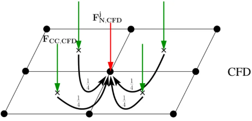
1. Conservative interpolation of the fluid loads located in the cell centers (CC) to the cell nodes (N) of the fluid domain (CFD→CFD, done in FASTEST-3D, see Fig. 2):

X

CFD nodes

F_N,CFD = X

cell centers

F_CC,CFD (14)

Since the cell centers (CC) are exactly located in the geometrical centers of the cell, it means that for an internal node not located at an edge the fluid load is equally distributed to its four neighboring cell nodes (N), i.e., a quarter to each node. At edges of the interface, this rule has to be adjusted accordingly.

CFD

FCC,CFD

1 4 1 4

1 4

1 4

F^j_N,CFD

Figure 2: Interpolation of loads from the cell centers (CC) located at the CFD–CSD interface to the nodes (N) of the CFD grid. Note: Both, CC and N lie in the same plane.

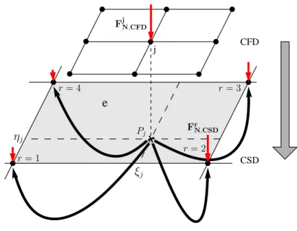
2. Conservative interpolation of the fluid loads from the cell nodes of the fluid domain to the grid nodes of the structure domain (CFD→CSD, done in CoMA, see Fig. 3):

X

CSD nodes

F_N,CSD = X

CFD nodes

F_N,CFD (15)

To achieve this, the fluid load F^j_N,CFD at the grid node j is split up to parts which are distributed to all nodes of the CSD element e, in which the fluid node j is found. The weighting is based on the shape function N_r^e of the CSD element e. It reads:

F^r_N,CSD = N_r^e(ξj, ηj)F^j_N,CFD (16) (ii) The calculated displacement vectors of the CSD nodes are transferred to the CFD nodes by using a bilinear interpolation. This interpolation is a consistent scheme for four–node elements with bilinear shape functions. A conservative interpolation as used to transfer pressure and viscous shear forces is not suitable here, because the displacements are not integral quantities.

Thus the final step of the interpolation procedure reads:

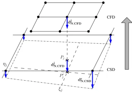
3. Bilinear interpolation of the displacements from the structure domaind^r_N,CSD to the cell vertices of the fluid domain (CSD→CFD, done in CoMA, see Fig. 4):

d^j_N,CFD =

4

X

r=1

N_r^e(ξ_j, η_j)d^r_N,CSD (17)

CFD

CSD j

e

F^j_N,CFD

r= 1

r= 4 r= 3

r= 2 P_j F^r_N,CSD

ηj

ξ_j

Figure 3: Transfer of loads from the fluid domain (CFD) to the structure domain (CSD).

Here, the resulting displacements in the fluid domain are denoted by d^j_N,CFD. They are obtained by the displacements of the structure domain d^r_N,CSD weighted by the shape functions N_r^e of the CSD element e, in which the fluid node j is found. Thereby ξj and ηj describe the local coordinates of the projection pointPj in the CSD element e.

CFD

CSD d^j_N,CFD

Pj

ξj

ηj

P_j^′

d^r_N,CSD d^j_N,CFD

Figure 4: Transfer of displacements from the structure domain (CSD) to the fluid domain (CFD).

The interpolation steps 2 and 3 are done in CoMA. This code coupling tool is based on the Message–Passing–Interface (MPI) and thus runs in parallel to the fluid and structure solver. The communication in-between the codes is performed via standard MPI commands using a special communicator for this purpose. Since the code parallelization in FASTEST- 3D and Carat++ also rely on MPI, separate communicators are introduced for each code.

Thus a hierarchical parallelization strategy with different levels of parallelism is achieved.

According to the CPU time requirements of the different subtasks, an appropriate number of processors can be assigned to the fluid and the structure part. Owing to the reduced structural models on the one side and the fully three–dimensional highly resolved fluid prediction on the other side, the predominant portion of the CPU time is presently required for the CFD part.

Hence in addition to the domain decomposition on the fluid and structure side, discipline decomposition is accomplished allowing the usage of modern multi–core architectures with their specific hierarchy of parallelism. Thus effective coupling with respect to high–performance computing is enabled.

4. Test Cases

A collaborative effort of the DFG Research Unit 493 (Bungartz et al., 2010) was the develop- ment of specific benchmark problems for validating various solution methods for fluid–structure interaction. In order to allow the application of a wide range of different coupling strategies and numerical schemes, the configuration considered is geometrically not very challenging and furthermore restricted to the laminar flow regime (Turek and Hron, 2006). One of these bench- mark cases, namely FSI3, is used in this study to validate the numerical methodology proposed.

The setup is described in § 4.1. To go beyond the limit of laminar flows and to test the FSI scheme in the turbulent regime applying LES, the setup of FSI3 was slightly adapted. The new configuration called FSI–LES is given in § 4.2

4.1. FSI Benchmark for Laminar Flow

The present FSI3 configuration (Turek and Hron, 2006; Turek et al., 2010) leans on an older

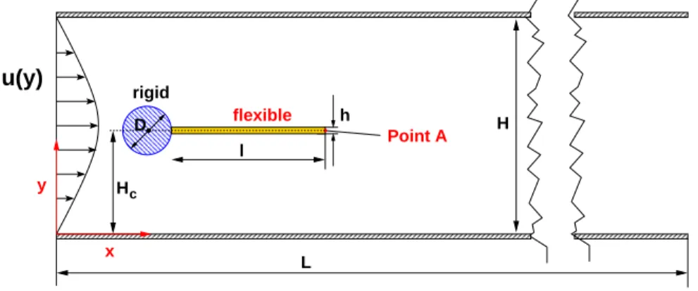
‘flow around cylinder‘ benchmark developed for testing CFD methods in the laminar flow regime (Turek and Sch¨afer, 1996). In order to extend the original CFD benchmark to a FSI test case, a flexible structure is attached to the back side of the cylinder (Turek and Hron, 2006). In a two–dimensional channel of length L/D = 25 and height H/D = 4.1 a fixed and rigid cylinder of diameterDis mounted as sketched in Fig. 5. The cylinder position is slightly off–centered, with the cylinder center located at 2Ddownstream of the inflow section and with a distance ofHc = 2D from the lower lateral channel wall. Providing dimensions the cylinder has a diameter ofD= 0.1 m. The fluid is assumed to be an incompressible Newtonian fluid with ρ^f = 1000 kg/m³. Based on a mean inflow velocity of u∞ = 2 m/s and a kinematic viscosity of ν^f = 0.001 m²/s a Reynolds number of Re = 200 is obtained. According to the analytical solution for a fully developed laminar channel flow, a parabolic velocity profile was set at the inflow given by

u(y) = 1.5u∞

y(H−y)

¡_H

2

¢2 . (18)

Besides the parabolic inflow condition (18) for the flow, no–slip boundary conditions should be applied at the channel walls, at the rigid front cylinder and at the flexible structure (Turek and Hron, 2006). At the outlet the conditions are not prescribed in Turek and Hron (2006).

Generally, a convective outflow boundary condition should be favored allowing vortices to leave the integration domain without significant disturbances (Breuer, 2002).

The elastic structure has a length of l/D = 3.5 and a thickness of h/D = 0.2. The structure is allowed to be compressible, and its deformations are significant. The material of the flex- ible structure is specified by the St. Venant–Kirchhoff material law (Belytschko et al., 2000) characterized by a Poisson’s ratio of ν^s = 0.4, a Young’s modulus of E = 5.6·10⁶ kg/(m s²) and a density of ρ^s = 1000 kg/m³. Consequently, the density ratio ρ^f/ρ^s is unity and the added–mass effect plays an important role. All nodes of the structure on the rigid cylinder are

assumed to be fixed. Contrarily, the nodes of the flexible structure are totally free at the free extremity.

L

H l

D h

Point A flexible

rigid

H_c

x y

u(y)

Figure 5: Setup of the computational domain for the FSI3 test case.

As a first step of a thoroughly carried out validation procedure, the single components (CFD and CSD solver) have to be addressed independently. For this issue, Turek and Hron (2006) defined the test cases CFD3 and CSM1 to CSM3, respectively. Both are briefly sketched and the results achieved will be shwon in § 6.1.1 and § 6.1.2.

Benchmark CFD3.

Assuming that the flexible structure in Fig. 5 is rigid, the FSI3 benchmark reduces to a pure CFD test case denoted CFD3 (Turek and Hron, 2006). The remainder of the test case and setup is kept unchanged. Thus the laminar two–dimensional flow around a cylinder with a kind of splitter plate at the backside mounted in a channel is considered for validation of the CFD code.

Benchmarks CSM1 to CSM3.

Similar to the validation of the CFD tool also the CSD tool is first validated in an uncoupled environment. For that purpose the benchmarks CSM1 to CSM3 (Turek and Hron, 2006) are taken into account. Based on the setup sketched in Fig. 5 solely the elastic beam without the surrounding fluid is considered here. In order to predict a deflection of the structure, a gravitational acceleration of g = 2 m/s² in negative y–direction is added. The CSM3 test is computed as a time–dependent case starting from the undeformed configuration while the tests CSM1 and CSM2 are the steady–state solutions. The material parameters are equal to those defined for FSI3 in §4.1 except the Young’s modulus which is reduced to E = 1.4·10⁶ kg/(m s²) for the cases CSM1 and CSM3.

4.2. FSI Benchmark for Turbulent Flow

For extending the coupled FSI3 case towards an appropriate test case for the turbulent flow regime (FSI–LES), several adjustments are necessary. These are required either to allow LES or to reduce the computational effort to a reasonable level.

First, the computational domain has to be extended to a three–dimensional geometry since turbulence is always 3–D and LES predictions can thus not rely on two–dimensional integration domains. Therefore, the computational domain has now a width of W/D = l/D = 3.5 in z–

direction. Thus the flexible structure is a square in the x–z–plane.

Second, owing to this three–dimensional extension of the domain, boundary conditions are required for the flow and for the structure. Thus, in spanwise direction periodic boundary

conditions are chosen for both disciplines. For the structure that implies that in the cross–

section (x–y plane) the same boundary conditions are used as in 4.1. Additionally, the z–

displacement of the nodes on the sides are forced to be zero. Due to periodic boundary conditions set in the fluid solver there are always two nodes of the sides (one in a plane and its twin in the other plane) which have the same load. These two nodes must have the same displacement in x– and y–direction.

Third, since the resolution of the boundary layers at the channel walls would require the bulk of the CPU time, the lateral channel walls are assumed to be slip walls. Thus the blocking effect of the walls is maintained without taking the boundary layers into account. Of course, on the structure, no–slip boundary conditions are used as in the laminar case. At the channel outlet again a convective outflow condition is specified to avoid reflections and disturbances (Breuer, 2002).

Fourth, as a direct consequence of the slip conditions at the channel walls, the inflow profile has to be modified and a constant velocity u∞ is now set at the inflow.

Fifth, in order to enter the turbulent regime, the Reynolds number is set toRe =u∞D/ν^f = 10⁴. For the pure cylinder the flow is in the sub–critical regime at this Reynolds number, where the boundary layer at the cylinder is still laminar and transition to turbulence takes place in the free shear layers behind the cylinder (Breuer, 1998, 2000). All other dimensions and properties of the fluid and the structure are kept unchanged.

Benchmark CFD–LES.

In order to initialize the coupled FSI–LES case and to check the LES prediction of the turbulent flow, in a first step the flexible structure is again assumed to be rigid as in the laminar case.

Thus, the FSI–LES benchmark reduces to a pure CFD test case denoted CFD–LES.

5. Numerical Setup

The predictions are carried out based on the numerical schemes described in § 2 and § 3. In the following specific settings are provided for both, laminar and turbulent cases separately.

5.1. FSI Benchmark for Laminar Flow including CFD3 and CSM1–3

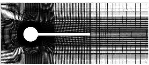
In order to allow a grid independence study for the laminar flow cases CFD3 and FSI3, a series of three block–structured grids was taken into account for the flow predictions. In the cross–section the grid is successively refined by a factor of two in both directions. The coars- est grid (2–D) depicted in Fig. 6 consists of about 27,000 control volumes (CVs). The next finer level, i.e. the medium grid, possesses about 90,000 CVs and the fine grid consists of about 360,000 CVs. In wall–normal direction the first cell center is located at a distance of

∆y/D = 6.925·10⁻³, 3.125 · 10⁻³ and 1.5· 10⁻³ from the flexible structure for the coarse, medium and fine grid, respectively. Owing to the grid stretching applied in wall–normal di- rection, the ratio between two successive grid levels is not exactly one half. For the structure the corresponding grid is kept fixed for all three FSI3 predictions (coarse, medium and fine).

It consists in total of 30 four–node shell elements. The same discretization is also applied for the preliminary structural tests CSM1 to CSM3.

Since for low Reynolds numbers the stability of explicit time–marching schemes is dominated by viscous effects, the time–step size has to be reduced with the refinement of the grid in order to stay in the stable limits². Therefore, time–step sizes of ∆tf = 10⁻⁴ s, (coarse grid), 5·10⁻⁵ s

2Since the FSI coupling scheme is mainly intended for high–Re flows within the LES context, this restriction solely applies to the present laminar test case.

(medium grid) and 10⁻⁵s (fine grid) are chosen to predict the flow field, respectively. Although in general different time–step sizes are possible for both solvers, presently this option is not implemented in the coupling tool CoMA. Hence in all cases considered the time–step size of the solver for the structure is adapted to the time–step size of the fluid solver, i.e., ∆ts = ∆tf. For time–stepping the structural solution the generalized–α method is applied with a spectral radius ̺∞= 0.8.

Within the coupled FSI prediction a constant underrelaxation factor of ω = 0.5 is considered for transferring the computed displacements from the structure domain to the fluid domain (see discussion in § 6.1.4). No underrelaxation of the fluid loads is necessary as mentioned in

§ 3.2. For this case, a linear first–order extrapolation (11) for the estimation of the structural displacements at the beginning of each time step is performed. The choice is already motivated in§ 3.2.

FSI convergence is reached if the L2 norm of the displacement differences according to eq. (10) drops below εF SI = 10⁻⁵. For that purpose in the mean about 10 FSI–subiterations are required. Tests were also carried out with a limit of εF SI = 10⁻⁴ and 10⁻⁶. For the former reasonable results but partially overlayed by minor perturbations on the lift and drag curves were obtained. For the latter the same results as forεF SI = 10⁻⁵ were noticed which motivates the current choice.

Finally, it should be noted that the present coupling algorithm was also tested as a loosely coupled scheme by setting the number of FSI–subiterations to zero. However, as expected the scheme becomes unstable after a few time steps owing to the artificial added–mass effect, see, e.g., Causin et al. (2005); F¨orster et al. (2007); F¨orster (2007).

X Y

Z

Figure 6: Coarse grid for the FSI3 test case in the x–y cross–section, about half of the computational domain in the wake region omitted.

5.2. FSI Benchmark for Turbulent Flow including CFD–LES

For the flow prediction based on LES (i.e., the cases CFD–LES and FSI–LES) a block–

structured grid with about 17 million CVs is used, whereas 48 CVs are applied in the spanwise direction. The grid points are clustered towards the rigid cylinder and the flexible structure using geometric stretching. The stretching factors are kept below 1.1 with the first cell center located at a distance of ∆y/D = 1.5·10⁻³ from the flexible structure. The prediction CFD–

LES for a rigid structure served as a source for the determination of time–averaged wall shear stresses on the cylinder and the structure. Based on that the averagey⁺ values are predicted

on the structure and found to be below 1, mostly even below 0.2. Thus, the viscous sublayer is adequately resolved. In contrast to the former case no grid clustering is required at the slip channel walls. The elastic plate is resolved by the use of 10×10 four–node shell elements.

For the turbulent case the restrictions concerning the time–step size are less restrictive as forecasted above. Thus a time–step of ∆tf = 10⁻⁴ s is chosen and again the same time–step size is applied for the structural solver based on the generalized–α method with ̺∞ = 0.8.

Again a constant underrelaxation factor ofω= 0.5 is considered for the displacements and the loads are transferred without underrelaxation. Based on the experiences with the second–order extrapolation in the laminar case, here solely the first–order extrapolation for the estimation of the structural displacements at the beginning of each time step is used. In accordance with the laminar case the FSI convergence criterion is set to εF SI = 10⁻⁵ for the L2 norm of the displacement differences according to eq. (10).

For the LES predictions the national supercomputer SGI ALTIX 4700³ was used applying in total 142 processors for the CFD part plus one processor for the coupling code and the CSD code, respectively.

6. Results

6.1. Validation of the Methodology based on Laminar Flow

In the following, first the results of the validation procedure for both subtasks (CFD and CSM) are briefly shown. Then the coupled laminar case FSI3 is discussed in more detail.

6.1.1. Benchmark CFD3

As mentioned above, replacing the flexible structure in Fig. 5 by a rigid plate, the FSI3 bench- mark reduces to the pure CFD test case CFD3 (Turek and Hron, 2006). It considers the laminar flow around a cylinder with a splitter plate at the backside. The comparison will be done for fully developed flow, and particularly for one full period of the oscillation. Forces exerted by the fluid on the whole submerged body, i.e. lift and drag forces acting on the cylinder and the beam structure together, are taken into account for comparison. Although unusual, in order to be consistent with the reference data (Turek and Hron, 2006) provided by a fully implicit FEM method with a coupled multigrid solver, the results are provided by dimensional quantities.

Furthermore, the forces are given per unit length since the problem is two–dimensional.

Despite the splitter plate behind the cylinder, vortex shedding occurs at Re = 200. The shed vortices travel downstream and interact with the structure (not shown here, see similar behavior for the flexible structure in Fig. 7). The time history of the lift force shows a sinusoidal signal where the mean value is not equal to zero due to the slightly off–centered position of the structure in the channel. To quantify the results for comparison purposes, the minimal and maximal values are provided in Table 1 for the three successive grids applied. It is obvious that the values of the minimal and the maximal lift converge step by step towards the reference data when the grid is refined consecutively. Regarding the corresponding frequencies of the oscillating lift force the predicted values are about 1% higher than in the reference case and that does not change with grid refinement. Since the scheme applied is second–order accurate in time and the time–step sizes are 50 to 500 times smaller than in the reference case, this minor deviation is still astonishing. As usual for the vortex shedding phenomenon past bluff bodies, the frequency of the drag force is doubled with respect to the lift force. Besides the absolute minimum and maximum the time history of the drag (not shown here) depicts a local

3http://www.lrz.de/services/compute/hlrb/

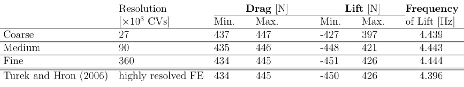
Table 1: Results of the CFD3 benchmark.

Resolution Drag [N] Lift [N] Frequency

[×10³ CVs] Min. Max. Min. Max. of Lift [Hz]

Coarse 27 437 447 -427 397 4.439

Medium 90 435 446 -448 421 4.443

Fine 360 434 445 -451 426 4.444

Turek and Hron (2006) highly resolved FE 434 445 -450 426 4.396

minimum and a local maximum. Table 1 provides the values of the absolute extrema. Again it is observed that the values of the present predictions converge towards the reference data when the grid is refined. Consequently, the grid refinement study was successful and the CFD solver is validated.

6.1.2. Benchmarks CSM1 to CSM3

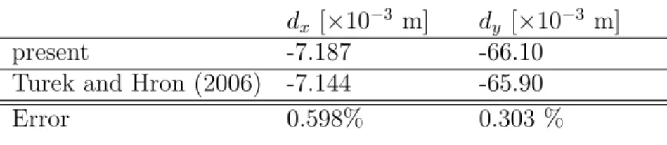
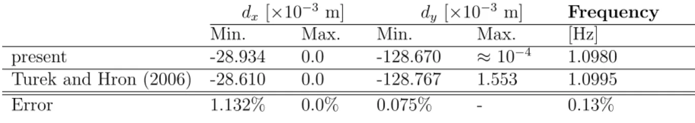
The next step is to validate the CSD tool in an uncoupled environment using the benchmarks CSM1 to CSM3 suggested by Turek and Hron (2006). The setup solely includes the elas- tic beam without the surrounding fluid. The tests CSM1 and CSM2 are steady–state cases, whereas CSM3 has to be computed as a time–dependent case starting from the undeformed configuration. Tables 2 and 3 summarize the predicted steady–state deflections in both direc- tions in comparison with the reference data (Turek and Hron, 2006). In all cases an error of less than 0.6% is found. Table 4 summarizes the comparison for the unsteady case CSM3 based on the minimal and maximal deflections and the frequency of the oscillation. A maximum deviation of about 1.1% is observed for the deflection in x–direction. The minimum deflection in y–direction fits well to the reference data, whereas for the maximal deflection a value larger than the initial position is provided in (Turek and Hron, 2006) which is hard to explain. The predicted frequency is in close agreement with the reference data. In conclusion, based on minor deviations observed also the CSD solver is successfully validated.

Table 2: Results of the CSM1 benchmark.

d_x [×10⁻³ m] d_y [×10⁻³ m]

present -7.187 -66.10

Turek and Hron (2006) -7.144 -65.90

Error 0.598% 0.303 %

6.1.3. Benchmark FSI3

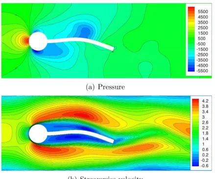
The natural extension of the previous case is to release the flexible structure again and to tackle the coupled FSI problem. Fig. 7 depicts contours of the pressure and the streamwise velocity at an arbitrarily chosen time instant. Similar as before vortex shedding is observed at the cylinder⁴. Vortices detach from the cylinder in an alternating manner. They travel

4See FSI3 videos in the online version of the paper!