HAL Id: hal-00943154
https://hal.archives-ouvertes.fr/hal-00943154
Submitted on 7 Feb 2014
HAL is a multi-disciplinary open access archive for the deposit and dissemination of sci- entific research documents, whether they are pub- lished or not. The documents may come from teaching and research institutions in France or abroad, or from public or private research centers.
L’archive ouverte pluridisciplinaire HAL, est destinée au dépôt et à la diffusion de documents scientifiques de niveau recherche, publiés ou non, émanant des établissements d’enseignement et de recherche français ou étrangers, des laboratoires publics ou privés.
Study of a transition in the qualitative behaviour of a simple oscillator with Coulomb friction
Elaine Pratt, Alain Leger, Xiang Zhang
To cite this version:
Elaine Pratt, Alain Leger, Xiang Zhang. Study of a transition in the qualitative behaviour of a simple oscillator with Coulomb friction. Nonlinear Dynamics, Springer Verlag, 2013, 74 (3), pp.517-531.
�10.1007/s11071-013-0985-6�. �hal-00943154�
Study of a transition in the qualitative behaviour of a simple oscillator with Coulomb friction
Elaine Pratt∗, Alain L´eger†, Xiang Zhang‡
Abstract
A simple mass-spring system is submitted to a constant force in addition to a periodic perturbation of rectangular wave shape. It has been obtained in a previous study that the range of the period-amplitude plane of this perturbation where the trajectories are sliding without jumps is divided into two parts, one in which there exist infinitely many equilibrium states and no periodic solutions, and another one where there exist periodic solutions and no equilibrium states. The present work focuses on the transition between these two parts. All along the transition line, there exists a single equilibrium state. Initial data out of equilibrium lead either to a periodic trajectory, or to a trajectory which tends to the equilibrium or to a periodic solution, either in finite time or at infinity.
Keywords Coulomb friction, equilibrium states, mass-spring systems, nonsmooth dynamics.
1 Introduction
This paper goes deeper into the investigation of the dynamics of a simple mass-spring system involving non regularized unilateral contact and Coulomb friction conditions. The investigation began by the set of equilibria which was immediately shown to have very specific features by comparison to those of classical dynamical systems. Two fundamental questions were addressed which continue to motivate theoretical works. The first one concerned stability. Classical stabil- ity analysis of the equilibrium states were performed both from the numerical [3] and theoretical [2] points of view, but it was soon observed that these analysis were not sufficient to take the actual dynamics into account. The observations led to a new notion of stability and to a con- jecture specially suited to the dynamics of systems involving Coulomb friction [7].
The second question was closely related to the qualitative analysis of dynamical systems, and can be stated in the following way: when a system involving unilateral contact and dry friction is submitted to an oscillating excitation, are we able to predict its answer by performing a partition
∗Laboratoire de M´ecanique et d’Acoustique - CNRS, 31, chemin Joseph Aiguier, 13402 Marseille Cedex 20, France. pratt@lma.cnrs-mrs.fr
†Laboratoire de M´ecanique et d’Acoustique - CNRS, 31, Chemin Joseph Aiguier, 13402 Marseille Cedex 20, France. leger@lma.cnrs-mrs.fr
‡Department of Mathematics and MOE-LSC, Shanghai Jiao Tong University, Minhang Campus, Shanghai 200240, China. xzhang@sjtu.edu.cn
of the period-amplitude plane of the excitation into different kinds of qualitative behaviours?
This was investigated in [8] where it was shown that the period-amplitude plane is essentially divided into three ranges. One range, for external forces of sufficiently small amplitude, is a horizontal strip, in which there exist everywhere infinitely many equilibrium states, no periodic solutions, and where any initial data out of equilibrium leads to a trajectory which attains an equilibrium in finite time. In a second range there exist no equilibrium states but the whole range contains periodic solutions, the number and the period of which depend on the period of the excitation. The latter range has a relatively intricate upper boundary above which the last range is such that there still exist periodic solutions, but all initial data lead to a trajectory which looses contact, so that the periodic trajectories involve jumps and shocks.
The present work continues the investigation of the period-amplitude plane, focussing on the transition between the range where there exist only equilibrium states and no periodic solutions and the range where there exist periodic solutions and no equilibrium states. We stress the fact that since the very beginning, all these analysis where possible due to a rigourous statement of the dynamics (see [10] and [6]) and to a proof that the corresponding Cauchy problem was well-posed [1].
The paper is concerned with sliding trajectories and is organized as follows.
Section 2 recalls the foundations of the present work, gives the dynamical system and the previous basic results concerning the partition of the period-amplitude plane.
Section 3 extends the investigation presented in the previous works and gives the proofs of the results which had simply been observed numerically before. It is shown that if the period of the external force is large enough, there exist infinitely many periodic solutions in addition to a single equilibrium state. Moreover, any initial data which does not belong to a periodic solution leads to a trajectory which converges to a periodic one, either in finite time or at infinity depending on the period of the excitation. At the end of this section we study the special case where the period of the external force is equal to an intrinsic value corresponding to a sliding phase to the right.
In Section 4, we consider smaller values of the period of the excitation, up to the limit of very high frequencies. Here there exists a single equilibrium state and no other periodic solutions.
The investigation is here relatively intricate and requires the range to be shared into several subintervals. It is shown that a trajectory tends generically to the equilibrium at infinity. But for any small enough period there exists a unique initial data such that the equilibrium is reached in finite time.
The whole analysis of these sections is performed using an excitation of a rectangular wave shape, in order to carry out analytical calculations as far as possible. So that the last section studies what remains of the transitions and of their qualitative meaning if the excitation is changed into a more classical harmonic one.
2 Preliminaries
2.1 The mechanical problem
We are studying a simple mass spring system which has been given in [5] for the analysis of the quasi-static evolution, and which is represented on Figure 1. A single mass m is connected to
a rigid frame by two springs, is submitted to an external force of components (Ft, Fn), and its motion in the plane is constrained by an obtacle which is the horizontal plane at the level zero.
The contact with the obstacle involves unilateral contact and Coulomb friction’s conditions. The corresponding contact and friction laws are kept all along this work without any regularization.
Let K= (Kt, Kn, W) be the stiffness matrix of the system of springs, µthe friction coefficient, (Rt, Rn) the reaction of the obstacle. The trajectories are the solutions to the following problem
Figure 1: The mass-spring system.
i) m¨ut=−Ktut+W un+Ft+Rt,
ii) mu¨n=−W ut+Knun+Fn+Rn, t >0, iii)
ut(0) =ut0, u˙+t(0) = ˙ut0
un(0) =un0, u˙+n(0) = ˙un0
iv) un≤0, Rn≤0, unRn= 0, v) µRn≤Rt≤ −µRn,
|Rt|<−µRn=⇒u˙t= 0,
|Rt|=−µRn=⇒ ∃λ≥0 s.t.u˙t=−λRt, vi) un(τ) = 0 =⇒u˙+n(τ) =−eu˙−n(τ), e∈[0,1].
(1)
In the case of sliding motions, that is when the trajectories do not involve loss of contact and jumps, inequalitiesiv) in system (1) reduce to un≡0, Rn≤0 so that system (1) reads
i) mu¨t=−Ktut+Ft+Rt,
ii) 0 =−W ut+Fn+Rn, t >0, iii) ut(0) =ut0, u˙t(0) = ˙ut0
iv) Rn≤0,
v) µRn≤Rt≤ −µRn,
|Rt|<−µRn=⇒u˙t= 0,
|Rt|=−µRn=⇒ ∃λ≥0 s.t.u˙t=−λRt,
(2)
where we observe that through equation (2-ii) we have a simple linear relation between ut and Rn which allows to deal indifferently with ut or Rn, and that in particular equations (2-i,ii,v) give:
either mu¨t=−(Kt−µW)ut+Ft−µFn, or mu¨t=−(Kt+µW)ut+Ft+µFn, for sliding respectively to the right and to the left, which we rewrite:
u¨t+ωα2ut=Ft−µFn,
¨
ut+ωβ2ut=Ft+µFn,
setting ωα2 := (Kt−µW)/mand ω2β := (Kt+µW)/m. All along this work we set Tα =π/ωα andTβ =π/ωβ for the half-periods of the sliding phases respectively to the right and to the left and we shall take mequal to 1.
2.2 Some preliminary results
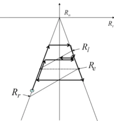
The set of equilibria has been investigated in several previous articles according to the values of the parameters µ, Kt, Kn, W, Ft, Fn (e.g. [8]). It has in particular been stated that the case when KtFn−W Ft >0 and Kt−µW > 0 can be considered as the most general in the sense that it involves all the difficulties that can be encountered separately in the other cases. LetA be the quantityKtFn−W Ft. We assume in the followingA>0 andKt−µW >0. In this case, the set of equilibria represented in the{Rt, Rn}plane, which is in general the intersection of the equilibrium equation (a straight line in the present case) and the Coulomb cone, is the thick line on Figure 2. A rectangular wave tangential force, of amplitude εand half-periodT, oscillating
Figure 2: Equilibrium solutions in the (Rt, Rn) plane.
between 0 and +ε, is now applied on the mass in addition to the constant force (Ft, Fn). Then the set of equilibria changes periodically from the thick line of Figure 3 to the dotted one.
Whether the corresponding intervals of normal components of the reaction at equilibrium have an empty intersection or not determines whether equilibrium states exist or not for such an oscillating load. The system under this periodic excitation behaves in a relatively complicated way, it may have equilibria, periodic solutions and non periodic solutions. A first investigation of the{T, ε} plane has been published in [8]. It has in particular been stated that there exists a critical valueε0 of the amplitude such that:
Statement 1. • i) Forε < ε0, there exist infinitely many equilibrium states for anyT, and any initial data out of equilibrium leads to a trajectory which reaches one of the equilibrium states in finite time.
• ii) Forε > ε0, there no longer exist any equilibrium states, but there exist periodic solutions for anyT, the number of these periodic solutions depends on T.
The critical value ε0 of the amplitude is given by ε0 = K2µA
t+µW , where A is the quantity involving the loading and stiffness parameters defined above.
Figure 3: The set of equilibria under oscillating loading. dotted line : when the tangential perturbation is equal to zero, full line : when the tangential perturbation is equal to ε.
- a - - b -
Figure 4: a - The single equilibrium forε=ε0, b - an example of trajectory in the (Rt, Rn) plane.
The present work deals with the transition between these two ranges. We shall moreover restrict our attention to sliding solutions, which means that we shall refer to initial data leading to loss of contact only as a boundary for the validity of the present study. Three points must be proved, which have essentially been observed from symbolic calculations and presented in [8]:
Statement 2. Forε= 2µA
Kt+µW there exists a single equilibrium solution for anyT. Moreover:
• i) whenT < Tα all the initial data different from the single equilibrium lead to trajectories which tend to the equilibrium,
• ii) when T > Tα there exist infinitely many periodic solutions and any initial data which does not belong to a periodic solution leads to a trajectory which goes to a periodic solution,
• iii) when T = Tα the set of periodic solutions is strictly larger than the set of periodic solutions obtained forT > Tα. Any initial data which does not belong to a periodic solution leads to a trajectory which tends to the periodic solution of largest orbit at infinity.
Throughout this paper, the figures are obtained by symbolic calculations using the following values for the coefficients and parameters of the problem
m= 1, µ= 0.5, and Fn= 2, Ft= 1, Kt= 2, W = 1,
so that in particularA= 3. (3)
3 The set of solutions when T is larger than T
α3.1 When T is strictly larger than Tα
When the amplitude ε of the perturbation is equal to ε0 = K2t+µAµW there exists a single equi- librium solution for any value of the half period T, let Ue be this equilibrium position. Other specific positions will be useful:
Uℓ is the equilibrium position in imminent sliding to the left when the perturbation is equal to ε0,
Ur is the equilibrium position in imminent sliding to the right with the perturbation equal to 0, Ud is the position such that all trajectories issued from (u0,0) with u0 < Ud loose contact.
Using equation (2-ii) and the fact that a trajectory shall no longer be a sliding trajectory (i.e. the mass looses contact) as soon as its reaction goes through the vertex of the cone, we easily get
Ue= Fn
W + −A+ε0W
W(Kt−µW) = Fn
W − A
W(Kt+µW) with normal reactionRe, Ud= Fn
W − 2A
W(Kt+µW) with normal reaction Rd, Uℓ = Fn
W + −A+ε0W)
W(Kt+µW) ≡ Ft+µFn+ε0
ωβ2 with normal reaction Rℓ, Ur = Fn
W − A
W(Kt−µW) ≡ Ft−µFn
ωα2 with normal reaction Rr.
(4)
We shall also use the quantityddefined as d=Uℓ−Ue= Fn
W + −A+ε0W
W(Kt+µW) −Ue= ε0
Kt+µW >0,
so that when necessary the symmetric ofUℓ with respect toUe will be simply Ue−d.
Remark 1. i) The numerical values chosen in (3) giveUr = 0.
ii) The inequalities Ur < Ue−d < Ue and Ud < Ue−d always hold. In particular inequality Ud < Ue−d results from the condition Kt−µW > 0 which has been referred to as the generic case and which is consequently assumed to hold all through this paper.
Let us recall the following lemma which shall be needed througout this section (the proof can be found in [7]):
Lemma 3.1. Let the loading be piecewise analytical and let {Rn}(t) be the set of normal com- ponents of the reactions at timetcorresponding to a strictly stuck equilibrium solution. Suppose thatA>0 and consider the trajectory of a sliding mass which satisfies problem (2).
If at an instant t∗ when the mass stops sliding its normal reaction R∗n belongs to the interior of {Rn}(t∗) then the mass shall remain in a strictly stuck equilibrium state as long as its normal reaction belongs to the interior of {Rn}(t) (i.e. in particular for any subsequent time if the external force does not change).
For example, when the external load changes periodically from (Ft, Fn) to (Ft+ε, Fn) with a period 2T,{Rn}(t) = [Re, Rℓ] fort∈[0, T[ and {Rn}(t) = [Rr, Re] fort∈[T,2T[ (see Figure 4-a).
We now use the notationuin place ofut(since we are studying sliding motions no confusion is possible). Let the external loading be such that ε = ε0 defined at statement 1. Then the qualitative behavior of the solutions to system (2) is given by the two following propositions.
Proposition 3.2. Let T > Tα, ε=ε0 andKt−µW >0 then any initial data(u0,u˙0) such that u0 ∈[Ue−d, Ue] and u˙0 = 0 leads to a periodic solution of period 2T.
Proof. The external load changes periodically from (Ft, Fn) to (Ft+ε0, Fn) with a period 2T. It is equal to (Ft+ε0, Fn) on [0, T[ and to (Ft, Fn) on[T,2T[. If u0 ∈[Ue−d, Ue] then Rn(Tα) belongs to [Re, Rℓ] and Lemma 3.1 implies that the mass shall remain motionless fort∈[Tα, T].
When the load changes it starts sliding to the left and once again Lemma 3.1 implies that the mass shall remain motionless for t ∈ [T +Tβ,2T]. So that for u0 ∈[Ue−d, Ue] the motion is governed by the following system:
¨
u+ω2αu=Ft+ε−µFn, t∈[0, Tα], u(0) =u0, u(0) = 0,˙
u(t) =u(Tα), u(t) = 0,˙ t∈[Tα, T],
¨
u+ω2βu=Ft+µFn, t∈[T, T +Tβ], u(T) =u(Tα), u(T) = 0,˙
u(t) =u(T+Tβ), u(t) = 0,˙ t∈[T +Tβ,2T].
(5)
A solution to system (5) is such that :
u(T) =u(Tα) =Ue+ (Ue−u0) andu(2T) =u(T+Tβ) =Ue−(u(T)−Ue) =u0,u(2T) = 0.˙ In other words the solution is 2T periodic.
Remark 2. i) On all the figures the use of the numerical values defined at equation (3) imply that the interval [Ue−d, Ue+d] is equal to[0.32,1.28] .
ii) Studying only the case of initial data with zero velocity may seem restrictive. In fact, in- troducing a nonzero initial velocity would not lead to important changes in the case of a linear stiffness matrix K. The case where unilateral contact and Coulomb friction is coupled with a nonlinear restoring force is much more intricate as can be seen in [9] where the study of the equilibrium states is to be found.
iii) Choosing u0 < Ue implies that the first phase of the motion is a sliding phase to the right. If
u0 ≥Ue then the first phase would be either motionless or sliding to the left but no other periodic solutions would be found.
Of course ifu0 < Ue−dthenRn(Tα) is greater thanRℓthereforeRn(Tα)∈/ [Re, Rℓ] so that the mass does not stay motionless in the time interval [Tα, T] and the motion is no longer governed by system (5). Whether in the{Rt, Rn}plane or in the phase space {ut,u˙t}, the set of periodic trajectories fills completely the inside of the domain bounded by the periodic trajectory of largest amplitude represented on Figure 5. Proposition 3.4 will prove how trajectories starting out of interval [Ue−d, Ue+d] behave and will also show that there are no other periodic solutions than those given by proposition 3.2.
Let us start by showing that all sliding trajectories enter the interval [Ur, Ue−d[ in finite time.
–1 0 1
0.5 1 1.5
a - In the{Rt, Rn}plane b - In the phase space
Figure 5: The maximal size periodic solution forε=ε0 andT > Tα.
Lemma 3.3. Let Kt−3µW > 0, and assume that the initial position belongs to the interval [Ud, Ur[ and the initial velocity is equal to 0. Then, for any T > Tα, the trajectory enters the interval [Ur, Ue−d[ in finite time.
Proof. We are considering a period of the excitation T =Tα+ηwith a givenη strictly positive.
Assume that after any trajectory involving knon periodic loops, the trajectory is at some out- of-equilibrium position uk on the left side of the cone and take this position to be the initial data at a timet= 0, then there is a sliding phase to the right, then the trajectory jumps to the right side of the cone and there is a sliding phase to the left, then the trajectory comes back to a new out-of-equilibrium position uk+1 on the left side of the cone which makes a complete loop. More precisely, letτ1,τ2,τ3,τ4 be successive times defined as:
- during a first sliding phase to the right, τ1 is the time when the perturbation is set toε0, - τ2 is the time when the velocity of the sliding phase to the right goes through zero, so that τ2
is the end of the sliding phase to the right,
- during the sliding phase to the left, τ3 is the time when the perturbation is set to zero, - τ4 is the time when the velocity of the sliding phase to the left goes through zero.
Figure 6: One loop of the orbit forT > Tα, with some particular values useful for the calculations We chooseuk ∈[Ud, Ur[ and ˙uk= 0 as initial data, and look for the solution of the system:
¨
u+ωα2u=Ft−µFn on (0, τ1)
¨
u+ωα2u=Ft−µFn+ε0 on (τ1, τ2)
¨
u+ωβ2u=Ft+µFn+ε0 on (τ2, τ3)
¨
u+ωβ2u=Ft+µFn on (τ3, τ4),
(6)
using the continuity of the position uand of the velocity ˙u at timesτ1,τ2,τ3. From system (6) we calculateuk+1:=u(τ4), where τ4 is such that ˙u(τ4) = 0:
uk+1 =Ue− q
(Ue−U−d)2+d2+ 2d(Ue−U −d) cos(ωβη), whereU is an abstract initial position defined in the following way:
1) assume the perturbation is equal toε0 since the origint= 0 instead of being set toε0 at time τ1,
2) then (U ,0) is the initial data which would lead to a trajectory which would coincide with the actual trajectory calculated in [τ1, τ2],
3) as represented on Figure 6, this means thatU is symmetrical ofu(τ2) with respect toUe. So that,
(Ue−uk+1)2 = (Ue−U)2−2d(Ue−U−d)(1−cos(ωβη)), from which we obtain
uk+1−U = 2d(Ue−U −d)(1−cos(ωβη)) (Ue−U) + (Ue−uk+1) .
IfU ≥Ur then asuk+1 is larger thanU,uk+1 obviously belongs to [Ur, Ue−d[. If not then uk+1−uk ≥uk+1−U ≥ 2d(Ue−Ur−d)(1−cos(ωβη))
(Ue−Ud) + (Ue−Ud) ,
and setting
δ = 2d(Ue−Ur−d)(1−cos(ωβη)) 2(Ue−Ud) >0 we have
uk+1−uk≥δ >0.
This implies that uk is larger than Ur as soon as kδ > Ur−Ud, that is at most after 2kT, therefore in finite time.
Proposition 3.4. Let T > Tα, ε = ε0 and Kt−µW > 0, then the trajectories issued from any initial positionu0∈/ [Ue−d, Ue+d]are not periodic, and have a qualitative behavior which depends onT in the following way:
• i) for any T such that Tα < T ≤ Tα +Tβ/2, all sliding solutions tend to the largest amplitude periodic solution at infinity,
• ii) for any T such that T > Tα +Tβ/2 all sliding solutions reach one of the periodic solutions in finite time.
Proof. According to the values given in equation (4) and to remark (2-iii), proving Proposition 3.4 amounts to investigating the behavior of any trajectory starting with a zero velocity and an initial position u0 such that
Ud< u0 < Ue−d. (7)
Thanks to Lemma 3.3, we restrict the proof of Proposition 3.4 to trajectories starting from initial positions in the interval [Ur, Ue−d[ with a zero velocity. Setting uk =u(2kT) it is easy to check that Lemma 3.1 implies that for all k, uk ∈[Ur, Ue−d[, so that τ1 = 0 in system (6) and we can easily calculateuk+1. We introduce the following notation: xk=Ue−uk.
• IfT ≥Tα+Tβ then ˙u(τ3) = 0 and the solution of system (6) gives:
xk+1=p
d2+ (xk−d)2−2d(xk−d), so that
xk+1 = (d−(xk−d))>0.
But as uk∈[Ur, Ue−d[ this implies that xk−d >0 so that xk+1−d=−(xk−d)<0,
therefore, for any initial position in [Ur, Ue−d[ one of the periodic solutions is reached after 2T. Such a trajectory is represented on Figure 7 in the{Rt, Rn} plane.
• IfT < Tα+Tβ the solution of system (6) gives:
xk+1 = q
d2+ (xk−d)2+ 2d(xk−d) cosωβ(T−Tα). (8) The behaviour of the sequence{xk}defined by equation (8) depends on whether cosωβ(T− Tα) is positive or negative so that there are two cases:
Figure 7: A trajectory starting from initial positions in the interval [Ur, Ue−d[ with a zero velocity for T ≥Tα+Tβ.
– i)When Tα < T ≤Tα+Tβ/2, then 0≤cosωβ(T−Tα)<1 and consequently xk > d=⇒x2k+1−d2>0 =⇒xk+1 > d.
We deduce that∀k xk> dso thatdis a lower bound for the sequence {xk}. On the other hand equation (8) implies that
x2k+1−x2k= 2d(d−xk)(1−cosωβ(T −Tα))<0, (9) which means that the sequence {xk} is decreasing. Therefore the sequence {xk} converges, and passing to the limit in equation (9) we obtain that it converges towards d, which establishes point i)of Proposition 3.4.
– ii)When Tα+Tβ/2< T < Tα+Tβ, then cosωβ(T−Tα)<0.
In this case there exists a subscriptk∗such thatxk∗≤d. In other words the trajectory converges in finite time to the periodic solution with initial condition (uk∗,0). Let us assume that this is not so, that is that for all k,xk > d. Then for the same reasons than in (i) equation (9) implies that the sequence {xk} converges towards d. But from equation (8) we have
x2k+1−d2 = (xk−d)2+ 2d(xk−d) cosωβ(T−Tα) so that
(xk−d)2+ 2d(xk−d) cosωβ(T −Tα)>0, ∀k or
(xk−d) + 2dcosωβ(T−Tα)>0, ∀k.
But this cannot be true for all k since the quantity 2dcosωβ(T −Tα) is given and strictly negative whereas xk converges to d. So that the assumption xk > d, ∀k is false and there exists k∗ such that xk∗ ≤d.
We can see on Figure 8 two trajectories starting from the same initial data calculated with the numerical values given at equation (3): the first one, for T large enough, attains one of the periodic solutions in finite time, in fact after a very small number of sliding oscillations (Figure 8-a), the other one, for smallerT, converges to the largest amplitude periodic solution at infinity (Figure 8-b).
–1 1
1 2
–1 1
1 2
a -T > Tα+Tβ/2 b -Tα< T ≤Tα+Tβ/2
Figure 8: Two nonperiodic trajectories forε=ε0andT > Tα.
3.2 Periodic solutions for T =Tα
This section focusses on point iii) of statement 2. As in section 3 the amplitude of the pertur- bation of the load is fixed at the value of the transition ε=ε0 = Kt2+µAµW. Here the position of the pointUd corresponding to the limit of sliding solutions is important. It is easily shown that Ud≤Ur if and only ifKt−3µW ≥0. The starting point is the following:
Proposition 3.5. Assume T =Tα andε=ε0 then any initial data (u0,u˙0) with u˙0 = 0 and
u0∈[max(Ur, Ud), Ue] (10)
leads to a periodic solution of period 2T.
Proof. Ifu0is chosen in [Ur, Ue] then the motion shall be governed by a system similar to system (5), except that asT =Tα the motionless phase during [Tα, T] in (5) does not exist so that the trajectory is the solution to:
¨
u+ωα2u=Ft+ε−µFn, t∈[0, Tα], u(0) =u0, u(0) = 0,˙
¨
u+ωβ2u=Ft+µFn, t∈[Tα, Tα+Tβ], u(Tα) =u(Tα), u(T˙ α) = 0,
u(t) =u(Tα+Tβ), u(t) = 0,˙ t∈[Tα+Tβ,2T].
(11)
A solution to system (11) is such that :
u(Tα) =Ue+Ue−u0 and u(2T) =u(Tα+Tβ) =Ue−(u(T)−Ue) =u0 with ˙u(2T) = 0.
In other words the solution is 2T periodic.
The set of initial conditions that give a periodic solution is larger than when T > Tα simply because here when T = Tα the normal reaction Rn(Tα) does not belong to [Re, Rℓ] if u0 ∈ [Ur, Ue−d[ so that there is no motionless phase. Comparing this set with the one obtained for the caseT > Tα we observe that again it fills completely a domain, either in the{Rt, Rn}plane or in the phase space, which is bounded by the maximal amplitude periodic solution, but this set is now strictly larger than forT > Tα. It is represented on Figure 9, where we stress the fact that the scales on both axis of Figures 9-a,b are the same as those used for Figure 5-a,b.
–1 0 1
0.5 1 1.5
a - In the{Rt, Rn}plane b - In the phase space (note that the scale is the same as on Fig 5-b)
Figure 9: The maximal amplitude periodic solution forε=ε0andT =TαwithUd < Ur. Remark 3. Following Remark 1, the interval given by equation (10) is not empty if and only if Kt−3µW >0. If Kt−3µW ≤0, there exist no non periodic sliding solutions. All the sliding trajectories are periodic, and any other trajectory involves jumps.
4 When T is smaller than T
αProposition 4.1. AssumeT < Tαandε=ε0, then any initial data such thatu0∈]Ud, Ue[ and ˙u0 = 0 leads to a trajectory which converges to the single equilibrium.
An elementary corollary of Proposition 4.1 is that, due to the well-posedness of the Cauchy problem, no periodic solution exists (except the trivial one which is the single equilibrium point).
The proof of Proposition 4.1 is carried out in several steps, it will establish that all the trajectories of sliding motion converge to the equilibrium, but depending on the period and on the initial data the convergence holds in finite time or at infinity.
Step 1. Let T < Tα/2. Then there exists an initial data u0 such that the trajectory arrives exactly at the equilibrium point Ue with a zero velocity after a finite number of oscillations of the external force and involves only sliding phases on the left side of the cone.
To establish this existence result we are going to explicit the trajectory by a direct construction.
As long as the reaction remains on the left side of the cone, the positionu(t) is smaller thanUe
and the velocity ˙u(t) is strictly positive, the successive phases of the motion are given by:
i= 0, ...n−1,
t∈ ]2iT,(2i+ 1)T] : u(t) =Ue+ (uo−Ue) cosωαt− ε0
α2
2i
X
j=1
(−1)jcosωα(t−jT), t∈ ](2i+ 1)T,(2i+ 2)T] : u(t) =Ue− ε0
α2 + (uo−Ue) cosωαt− ε0
α2
2i+1
X
j=1
(−1)jcosωα(t−jT), (12) where the numbernof oscillations is associated with the period T of the load by:
Tα
2n+ 1 ≤T < Tα
2n−1. (13)
Consequently for any given half-period T in ]0, Tα/2], we can calculate from equation (12) an intial data (u0,0) such that the trajectory leads to the equilibrium Ue with zero velocity after noscillations (obviously a trajectory can reachUewith a zero velocity during the interval [0, T] only in the trivial case u0 =Ue). An example of such a trajectory is represented on Figure 10 forn= 7.
0 0.2 0.4
0.2 0.4 0.6 0.8
Figure 10: An example of trajectory represented in the phase space converging to the single equilibrium in finite time.
Let us give the fully explicit corresponding calculations in the case T =Tα/4, i.e. n= 2 from equation(13). This implies that the velocity can be zero for the first time at some ˜t∈ ]3T,4T] given by
tanωα˜t= sinωαT−sin 2ωαT+ sin 3ωαT
cosωαT −cos 2ωαT+ 3 cosωαT +αε02(u0−Ue)
and time ˜t will be the final point of the trajectory if u(˜t) =Ue, which gives the initial data for such a trajectory
˜
u0 =Ue−ε0
α2
cos 2ωαT(2 cosωαT −1) +
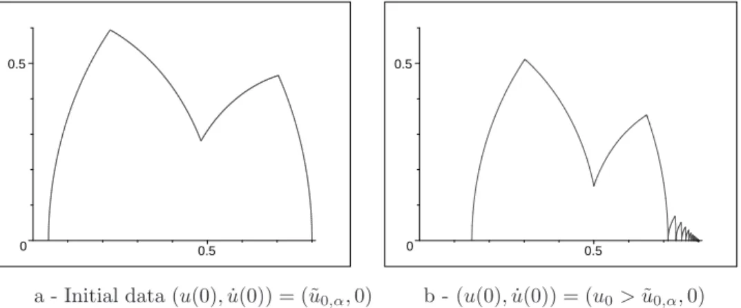
cos22ωαT(2 cosωαT −1)2−4 cosωαT(cosωαT −1)1/2 . From now onwards, we denote by ˜u0,αsuch an initial position to stress the fact that it corresponds to sliding phases to the right (and accordingly ˜u0,β will denote an equivalent initial position of sliding phases to the left, when necessary). The corresponding trajectory is represented Figure 11-a.
Step 2. LetT be a given half-period of the force in]0, Tα/2], and(˜u0,α,0)the initial data leading to a trajectory which reaches the equilibrium Ue in finite time for this period. Then, any initial data(u0,0) withu0∈ ]˜u0,α, Ue[leads to a trajectory which converges to Ue at infinity.
0 0.5
0.5 0
0.5
0.5
a - Initial data (u(0),u(0)) = (˜˙ u0,α,0) b - (u(0),u(0)) = (u˙ 0>u˜0,α,0)
Figure 11: One trajectory, here represented in the phase space, converges to the single equilibrium in finite time while the other converges to the equilibrium at infinity.
Proof. The proof of Step 2 is based upon the following result:
Lemma 4.2. Let T ∈ ]0, Tα/2]and an initial data (u0,0) such that Ue−u0 is strictly positive and satisfies the following inequality
Ue−u0 < 1 + tan2ωαT
2αε02 cosωαT , (14)
then the trajectory involves only sliding phases to the right which pile up at the left of Ue. proof. Let us first observe that inequality (14) implies that starting from a point u0 att = 0, the velocity will be equal to zero at some time t1 in ]T,2T[. So that the motion is governed by
t∈ [0, T] : u(t) =Ue+ (u0−Ue) cosωαt, t∈ [T, t1] : u(t) =Ue− ε0
α2 + (u0−Ue) cosωαt+ ε0
α2 cosωα(t−T), t∈ [t1,2T] : u(t)≡u(t1).
(15)
Of course we haveu1:=u(t1)> u0. Let thenuk−1 :=u(tk−1) be a point which is at equilibrium when the perturbation is equal to zero and from which a motion starts sliding to the right when the perturbation is set to ε0, and take (uk−1,0) as initial data. Inequality (14) implies that the trajectory involves only equation (15) so that we obtain the timetkand the positionuk:=u(tk) when the velocity is equal to zero again:
tanωαtk= sinωαT
cosωαT+αε02(uk−Ue), uk=Ue−α2
ε0
+ε20
α4 + (uk−1−Ue)2+2ε0
α2 (uk−1−Ue) cosωαT1/2
.
(16)
We have then defined a sequence {uk} from equation (16). The sequence {uk} is shown to be such that uk+1 > uk, and uk+1 < Ue and we easily check that it converges to Ue, which completes the proof of Lemma 4.2. Step 2 follows as a simple corollary. An example of such a case is represented on Figure 11-b, which is interesting to be compared to 11-a. The meaning of this comparison is that generically the convergence to equilibrium holds at infinity, but there exists particular values of the initial data for which the convergence holds in finite time, only two oscillations in the example of Figure 11-a.
Step 3. LetT be a given half-period of the external force, withT < Tα/2and(˜u0,α,0)the initial data leading to a trajectory which reaches the equilibriumUe in finite time for this period. Then, any initial data (u0,0)withu0 ∈ ]Ud,u˜0,α[leads to a trajectory which jumps to the other side of the cone and converges to Ue.
Proof. We recall that the special position Ud has been defined in equation (4) as the position such that all trajectories issued from (u0,0) withu0< Udloose contact. The sketch of the proof is then the following: at first, we observe that as soon as u0 ∈ ]Ud,u˜0,α[, the trajectory sliding to the right goes beyond the equilibrium Ue and, when its passes through zero, jumps to the other side of the cone. Secondly, as mentionned in Step 1, a position ˜u0,β such that a trajectory starting from (˜u0,β,0) involves only sliding phases to the left and reaches the equilibrium in finite time, does exists if T < Tβ/2. Thirdly we show that any trajectory starting from (u0,0) with u0 ∈ ]Ud,u˜0,α[ either enters the interval [˜u0,α,u˜0,β] in finite time if T < Tβ/2, or enters the interval [˜u0,α, Ue[ in finite time if not. From step 2, this implies the generic convergence at infinity toUe. Figure 12 represents an example of this convergence.
0 1
1
Figure 12: The trajectory enters the interval [˜u0,α,u˜0,β] in finite time and converges towards Ue at infinity.
Step 4. The range T ∈]Tα/2, Tα[ must be shared into two parts. We shall present the proof only in one case.
• (Tα+Tβ)/2< T < Tα: The trajectory always oscillates around Ue and converges to Ue at infinity; moreover the closer T is to Tα, the slower the convergence is.
The proof of this point stems from the fact that forT larger than (Tα+Tβ)/2 the motion stays at rest during the time interval [(Tα+Tβ)/2,2T] up to the time when the perturbation is set to ε0 again. This implies that each loop starts from an equilibrium position with a zero velocity, and this situation does not depend on the amplitude so that no phase difference accumulates from one loop to the next and only the value Tα−T determines the rate of convergence towards Ue. The trajectory is represented on Figure 13-a. This can be written explicitely.
Proof. Assume the initial data is (u0,0) and the trajectory starts a sliding phase to the right at time t=0 when the perturbation is set toε0. Then the trajectory is built piecewisely
as the solution to the following system:
¨
v1+ωα2v1 =Ft+ε0−µFn, t∈]0, T[, v1(0) =u0, v˙1(0) = 0,
¨
v2+ωα2v2 =Ft−µFn, t∈]T,ˆt[, v2(T) =v1(T), v˙2(T) = ˙v1(T), where ˆt such that ˙v2(ˆt) = 0.
¨
v3+ωβ2v3 =Ft+µFn, t∈]ˆt,ˆt+Tβ[, v3(ˆt) =v2(ˆt), v˙3(ˆt) = 0,
(17)
where the part v3 involves only sliding to the left while the external force remains equal to zero. The end of this phase is a rest position up to the time 2T when the perturbation is set toε0 again. Through classical elementary calculations we get v2(ˆt) as a function of u0, and the arrival position of the loop:
v3(ˆt+Tβ) :=u1=Ue−(v2(ˆt)−Ue). (18) Of course these calculations can be changed into those of a loop starting at (uk,0) and arriving at (uk+1,0). For all k, let us introducedk:=Ue−uk . Then equation (18) gives
dk+1= s
d2k+ ε20 ωα4 − 2ε0
ω2αdkcosωαT − ε0
ω2α, (19)
Since (Tα +Tβ)/2 < T < Tα we have that π2 < ωαT < π, so that equation (19) implies dk+1 < dk. The sequence {dk} has a lower bound which is zero, and passing to the limit in equation (18), we obtain the convergence of the trajectory toUe at infinity.
• Tα/2< T <(Tα+Tβ)/2: the trajectory is less smooth, but still converges toUe.
The difference with the case (Tα +Tβ)/2 < T < Tα is that we now have ˙u(2T) 6= 0 which implies that instead of having loops which all start at some data (uk,0), so that all the loops were solution of the same system with formally the same initial data, there is now a phase difference which accumulates at each loop between the trajectory and the loading. We can nevertheless, through calculations slightly more complicated that the previous ones, prove that the trajectory converges to Ue. The rate of convergence can be non uniform, but is more or less stronger depending on whether T is close to Tα/2 or to (Tα+Tβ)/2. An example of this last case is represented on Figure 13-b.
5 Concluding remarks: towards a more general excitation
This short concluding section can be taken on the one hand as an introduction to the genericity of the results of the investigation, and on the other hand as a useful complement to the qualitative analysis presented in [8]. The loadingsFt(t) andFn(t) are still taken of the form:
Ft(t) =Ft+Pt(t) and Fn(t) =Fn+Pn(t),
where Pt(t) and Pn(t) are respectively a tangential perturbation and a normal one, and we still restrict our attention to the case of a tangential perturbation, but we now choose Pt(t) = εsin(γt). We do not give theoretical results, but only numerical ones obtained by symbolic or numerical calculations.
0
1
–0.5 0 0.5 1
0.5 1
a - convergence at infinity for (Tα+Tβ)/2< T < Tα
b - convergence at infinity for Tα/2< T <(Tα+Tβ)/2
Figure 13: Two trajectories represented in the phase space for T2α < T < Tα.
5.1 The transition
We first present the two main qualitative features:
• The exact value of the amplitude for the transition is not affected.
As it was done on Figure 3 the set of equilibrium solutions can still be represented in the (Rt, Rn) plane. We deduce that whenε= (µA)/Kt the set{Rn}(t) reduces to a single point, so that the set of normal component of the reactions at equilibrium is a non zero measure interval when ε <(µA)/Kt and an empty set whenε > (µA)/Kt. For example in the case of the numerical values given at equation (3) we obtain (µA)/Kt= 0.75, which would also be the value obtained with a rectangular wave tangential force oscillating between−εand +ε.
• The qualitative meaning of the transition is not affected.
The transition shares the part of the {period−amplitude} plane where the trajectories do not loose contact into two parts, the lower one where non periodic solutions exist but infinitely many equilibrium states do, and the upper one, where periodic solutions exist but equilibrium states no longer do.
5.1.1 When ε is small enough
In this case the set{Rn}(t) is a nonzero measure interval. The existence of an infinity of equilib- rium solutions is then a straightforward consequence of Lemma (3.1) no matter the perturbation, whether of rectangular or sinusoidal wave shape. But it is interesting, both from the point of view of a constructive proof of the existence of equilibrium states and of specific notions of stability, to look at the trajectories starting from any initial data out of equilibrium. We still observe that all the trajectories go to equilibrium and an equilibrium state is always reached in finite time. Numerical simulations have been performed for different values of the frequencyγ. The qualitative behavior represented on Figure 14 is very close to that of the case where the perturbating load was a rectangular wave, as studied in [8].
–0.1 0 0.1 0.2 0.3 0.4
–0.2 0.2 0.4 0.6 –1
–0.5 0 0.5 1 1.5
–0.5 0.5 1 1.5
ε= 0.6 andγ= 0.4 ε= 0.6 andγ= 1.2
Figure 14: Evolution in the phase space (ut,u˙t) whenε= 0.6 5.1.2 When ε is large enough
In this case there no longer exist stationary solutions. However we observe the existence of periodic solutions of different types. Again this situation is close to the case where the external
–0.3 –0.2 –0.1 0 0.1 0.2 0.3
0.4 0.5 0.6 0.7 0.8 0.9
–0.15 –0.1 –0.05
0 0.05 0.1 0.15
0.4 0.5 0.6 0.7
a -ε= 1 andγ= 0.4 b - ε= 1 andγ= 0.2
Figure 15: Evolution in the phase space (ut,u˙t) whenε= 1
perturbation was a rectangular wave, as can be seen on Figures 15-a,b. Nevertheless, some differences appear since the trajectory represented on Figure 16-a is slightly more complicated than what had been obtained before at the same points of the {period−amplitude} plane.
Moreover, the complexity seems to be increasing forεsufficiently large and large periods, which had never been observed with the rectangular wave. An exemple is given on Figure 16-b.
5.2 The behaviour on the transition
Here it seems that there is a qualitative difference with the case of the rectangular waves. The main result of this numerical investigation is the following:
• Whatever the frequency of the oscillating perturbation, the trajectory tends to the single equi- librium at infinity.
Two examples of trajectories are represented on Figure 17.
–0.06 –0.04 –0.02 0 0.02 0.04 0.06 0.08 0.1
0.4 0.45 0.5 0.55 0.6 0.65
–0.1 0.1 0.2 0.3
0.5 1 1.5
a -ε= 1 andγ= 0.1 b - ε= 2.8 andγ= 0.1
Figure 16: Evolution in the phase space (ut,u˙t) for large periods
Again Figures 17-a,b look very much like those obtained in Section 4. But here, whatever the
–2 –1 1 2
–1 –0.5 0.5 1 1.5 2
0 0.05 0.1 0.15 0.2
0.2 0.25 0.3 0.35 0.4 0.45
a -ε= 0.75 andγ= 1.2 b - ε= 0.75 andγ= 2.4 Figure 17: Evolution in the phase space (ut,u˙t) whenε= 0.75
value of T on the transition line, we obtain only these two different types of trajectories. In the case of the rectangular wave these trajectories represent the qualitative dynamics only when T < Tα. When T > Tα, a rectangular wave leads to trajectories which no longer converge to the single equilibrium. They are either periodic or converge towards a periodic trajectory. This result of non existence of periodic solutions on the transition line in the case of a sinusoidal excitation must be handled with care since it only follows from numerical experiments for the moment, but it is an important qualitative point, which suggests further works in these lines.
References
[1] P. Ballard and S. Basseville. Existence and uniqueness for dynamical unilateral contact with Coulomb friction: a model problem.Mathematical modelling and Numerical Analysis, Vol. 39, 57–77, 2005.
[2] S. Basseville and A. L´eger. Stability of equilibrium states in a simple system with unilateral contact and Coulomb friction.Archive Appl. Mech., Vol. 76, 403–428, 2006.
[3] S. Basseville, A. L´eger and E. Pratt. Investigation of the equilibrium states and their stabil- ity for a simple model with unilateral contact and Coulomb friction, Archive Appl. Mech., Vol. 73, 409-420, 2003.
[4] M. Jean. The nonsmooth contact dynamics method.Computer Methods Appl. Mech. Engn, Vol. 177, 235–257, 1999.
[5] A. Klarbring. Examples of non-uniqueness and non-existence of solutions to quasistatic contact problems with friction.Ing. Archives, Vol. 60, 529-541, 1990.
[6] J.J. Moreau.Unilateral contact and dry friction in finite freedom dynamics. In Moreau J.J., Panagiotopoulos P.D. (Eds), Nonsmooth Mechanics and Applications, CISM courses and lectures 302, Springer-Verlag, Wien-New York, 1988.
[7] E. Pratt, A. L´eger and M. Jean. About a stability conjecture concerning unilateral contact with friction.Nonlinear Dynamics, Vol. 59, 73-94, 2010.
[8] A. L´eger and E. Pratt, Qualitative analysis of a forced nonsmooth oscillator with contact and friction,Annals of Solid and Structural Mechanics, Vol. 2, 1-17, 2011.
[9] A. L´eger, E. Pratt and Q.J. Cao, A fully nonlinear oscillator with contact and friction, Nonlinear Dynamics, Vol. 70, 511-522, 2012.
[10] M. Schatzman, A class of differential equations of second order in time,Nonlinear Analysis, Vol. 2, 355-373, 1978.