[PENDING] THÈSE Docteur UniversitédeGrenoble LuizFernandoZANINI FrédéricDUMAS-BOUCHIAT Bio-Mag-MEMSautonomesbaséssurdesaimantspermanents GilbertREYNE

(1)

THÈSE

pour obtenir le grade de

Docteur

_{de l’}

Université de Grenoble

Spécialité : Génie Electrique Arrêté ministériel : 7 août 2006

Présentée par

Luiz Fernando ZANINI

Ingénieur Matériaux par l’Université Fédérale de Santa Catarina, Brésil

Thèse dirigée par

Gilbert REYNE

^et

co-encadrée par

Frédéric DUMAS-BOUCHIAT

préparée au sein du Laboratoire de Génie Electrique de Grenoble

et de l’Institut Néel

Ecole Doctorale: EEATS - Electronique, Electrotechnique, Automatique, Télécommunication, Signal

Bio-Mag-MEMS autonomes basés sur des aimants permanents

Thèse soutenue publiquement le 18 février 2013 devant le jury composé de :

Dr. Anne-Marie GUE (Rapporteuse) Dr. Paulo WENDHAUSEN (Rapporteur) Dr. Stéphanie DESCROIX (Examinatrice) Dr. Marie FRENEA-ROBIN (Examinatrice) Dr. Gilbert REYNE (Directeur de thèse)

Dr. Frédéric DUMAS-BOUCHIAT (Co-encadrant) Dr. Nora DEMPSEY (Invitée)

(2)

(3)

Abstract

The range of applications for magnetic micro- and nano-particles is constantly expanding, in particular in medicine and biology. A number of applications involve particle trapping and deviation under the effect of a magnetic field and field gradient. In most publications, the required magnetic fields are produced either using soft magnetic elements polarized by an external magnetic field, electromagnets or bulk permanent magnets.

Micromagnets produce high fields and favor autonomy and stability while downscaling leads to an increase of field gradients. The challenge is to produce good quality, hard magnetic films in the range of 1 to 100 µm both in thickness and lateral dimensions and to integrate them into a Bio-Mag-MEMS.

Physical vapor deposition (triode sputtering) is used to prepare high quality rare earth magnets in thick ﬁlm form. In order to obtain ﬁeld gradients in the lateral directions, three techniques have been developed:

• Topographic patterning, in which the ﬁlm itself is patterned either by sputtering onto pre-etched substrates or by etching the magnetic ﬁlm.

• Thermo-magnetic patterning, which exploits the temperature dependance of coercivity to locally reorient the magnetization.

• Micro magnetic imprinting, which consists of organizing magnetic powder with the aid of the above-cited magnets, then embedding the powder into a polymeric matrix.

Such micro-magnets are autonomous, having no requirements for a cumbersome external ﬁeld source nor power supply.

Here we demonstrate the potential to develop autonomous devices based on micromagnet arrays. Controlled positioning using superparamagnetic particles as a model is shown at ﬁrst.

Then, the magnet arrays are used to study endocytic processes using magnetically labelled biological elements.

In a step towards device integration, microﬂuidic channels are produced above the magnet arrays. Magnetic and non-magnetic particles are pumped through the devices and precise positioning, as well as guiding and sorting are performed. High purity is obtained in the sorted solutions.

The good results obtained in the development of micromagnetic ﬂux sources, integration into microdevices and particle/cell handling and sorting indicate the high potential of this work for actual biological and medical applications. Moreover, the biocompatibility and autonomy of such devices allow their use in micro-total-analysis systems, point-of-care or implantable devices.

(4)

(5)

Résumé

Les micro et nano billes magnétiques sont de plus en plus utilisées en Biologie et en Médecine, pour une large gamme d’applications. Plusieurs applications utilisent le piégeage et le guidage de ces billes sous l’eﬀet d’un champ et d’un gradient de champ magnétique.

Dans la plupart des applications le champ magnétique est macroscopique, créé par un aimant ou un électro-aimant. L’intégration plus poussée est souvent envisagée, dans les articles scientiﬁques, par des microbobines ou par des éléments magnétiques doux. Ceux-ci doivent alors être polarisés par un champ externe (de nouveau, un électroaimant ou un aimant).

Les micro-aimants mis au point à l’Institut Néel permettent d’obtenir les mêmes inductions que les meilleurs aimants du marché et, par conséquent, de par la réduction d’échelle, des gradients de champ intenses. Ils sont, de plus, favorables à l’autonomie et à la stabilité du système. Le déﬁ est de produire de bonnes couches magnétiques avec des dimensions de l’ordre de 1 à 100 µm et de les intégrer à des Bio-Mag-MEMS.

Le dépôt physique par phase vapeur (pulvérisation cathodique triode) est utilisé pour le dépôt de ces aimants de haute qualité, en couche épaisse, et à base de terres-rares. Dans le but d’optimiser les gradients latéraux des champs magnétiques, trois techniques ont été développées:

• Le topographic patterning, dans lequel une couche est structurée géométriquement, soit par dépôt sur un substrat pré-gravé, soit par gravure humide après le dépôt.

• Le thermo-magnetic patterning, qui exploite la dépendance thermique de la coercivité pour réorienter localement l’aimantation de la couche.

• Le micro magnetic imprinting, qui consiste à organiser des particules magnétiques à l’aide des aimants mentionnés ci-dessus et, ensuite, de les noyer dans une couche polymérique.

Les micro-aimants présentent l’avantage, majeur pour un microsystème, d’être autonomes. Ils ne nécessitent pas de source externe de champ magnétique, ni d’alimentation électrique. Lors de ces travaux, nous développons des prototypes de microsystèmes fluidiques autonomes basés sur des réseaux de micro-aimants. En premier lieu, la capture par attraction et le positionnement controllé, en utilisant des particules superparamagnétiques comme modèle. Puis, l’étude de phénomènes d’endocytose à l’aide d’éléments biologiques marqués magnétiquement. Dans le but de passer à l’intégration des systèmes, des canaux microfluidiques sont développes sur les réseaux magnétiques. Des particules magnétiques et non-magnétiques sont introduites dans les canaux et leur positionnement, guidage et tri sont réalisés. L’analyse des solutions triées indique une haute efficacité du système.

Les résultats obtenus lors du développement de ces micro-sources de champ magnétiques et de leur intégration dans des microsystèmes, ainsi que la manipulation et tri de particules, démontrent le grand potentiel de ces recherches pour des applications grand public à des systèmes biologiques et médicaux. De plus, la biocompatibilité et l’autonomie de ces systèmes permettent leur utilisation dans des microsystèmes d’analyse totale (µTAS), des systèmes point-of-care (POC) et des implants biomédicaux, potentiellement jetables et bas coût.

(6)

(7)

Introduction

The curiosity and the need to understand and handle the tiny constituents of everything has been present among the humankind for millennia. From the hand-held magnifier, to the optical microscope and then to the scanning and transmission electron microscopes, knowledge of what things are made of have dramatically increased. The human body, for instance, is today known at different levels: organs, tissues, cells, constituents of cells, DNA, individual nucleotides. Once each of these parts and their functions are known, the challenge is to manipulate them so that they can perform specific functions at specific sites. Obviously, the human body is not the only subject of interest. Chemical reactions, Micro-Electro-Mechanical-Systems (MEMS), microbiology, etc., can all benefit from the ability to manipulate the world at low-scale.

A ﬁeld of research which is rapidly expanding concerns micro and nanoparticle handling.

These particles can have a vast range of properties and functional compounds added to their surfaces. The techniques used to produce the particles are, themselves, a research ﬁeld. The goal is to obtain narrower distributions in size, with optimized and reproducible properties and expand the list of available functions a particle can have. The success of these tiny objects can be observed, for example, by the numerous commercial kits which involve the use of particles for bio-assays or to perform sorting of particle-labelled objects (Miltenyi Biotec, DiagnoSwiss, etc.).

Diﬀerent techniques based on various physical, chemical and biological phenomena can be used to handle objects at the micro and nanoscale. All these techniques present a set of advantages and drawbacks and are more or less susceptible to integration in micro-devices.

For instance, dielectrophoresis can be used to act on several particles at once, or on a single particle, and can be easily integrated to a MEMS. However, this technique requires a set of conditions to operate properly (salinity of the medium, balance of responses between the medium and the object, etc.). Optical tweezers can also act on single or multiple objects with very high precision, but are much more diﬃcult to integrate. The ﬁnal device often requires a large amount of side-equipment, rendering impossible the development of an autonomous and transportable device. The list goes on and on, with electroosmosis, acoustics, thermal actuation...

Giving magnetic properties to an object can increase its potential applications.

Contactless actuation allow the manipulation of magnetically labelled objects without direct interference. Magnetic Resonance Imaging (MRI), for instance, is a technique which uses a large number of these particles and their magnetic response to study the internal parts of a subject. Magnetic particles can also be used to label individual objects, which can be then manipulated individually or as a group.

Magnetic separation devices have been developed and are commercially available. The use of bulk magnets for this purpose is evident, since they are a part of our everyday life.

However, it is not evident to all that the force created by these large magnets on very small objects can be very weak. The force is, actually, proportional to both the magnetic ﬁeld and the field gradient they produce, thus, a variation of the ﬁeld in space is of foremost

(12)

importance. Unfortunately, the relevant ﬁeld gradients of bulk magnets are restricted to a limited zone around its edges, and extremely close to it. For practical cases, such magnets fail to attract a very important part of the magnetic particles, especially if those are nano-scaled.

Using downscaled permanent magnets can signiﬁcantly enhance particle attraction while keeping the advantage of an autonomous magnetic ﬂux source. However, very few reports about it can be found in the literature. The reason is simple: when it comes to developing micro-magnets with the standard techniques of fabrication, one has to choose between

• obtaining high quality magnetic properties and

• precisely controlling the magnet’s dimensions.

It is quite straightforward to conclude that a high performance micro-object handling device cannot be developed if these two items are exclusive. Despite of the great potential of micro-magnets, little advances have been done worldwide in this ﬁeld. Micro-magnets nowadays are usually ferromagnetic thin ﬁlms based on a two-element iron alloy, or high-performance micro-particles arranged with poor control of particle packaging or dimensions.

The alternatives found for this problem are the use of electromagnets and soft micro-magnets. The magnetic field generated by an electromagnet is easily predictable and controllable. Moreover, their fabrication can be easily adapted to the standard micro-fabrication techniques. The advantages they present are the modulation of the field they produce and the possibility to have a zero field condition, if needed. On the other hand, they present two major drawbacks: Joule heating generated by the required electric current, and the need for external power supply. Soft magnets do not produce heat. However, their field is only generated when they are polarized by an external field, which implies a bulk magnet or an external electromagnet. Turning the field on and off is also possible, though it is not easily modulable. These two alternatives allow actuation at the micro-scale, but the integration to small devices is hardly achievable.

∗ ∗ ∗

In Institut Néel, more precisely in the Micro & Nano Magnetism (MNM) group, high quality magnets in the micrometer range are being developed these last 6-7 years.

These magnets are deposited by triode sputtering onto silicon wafers - thus, integration to microsystems is improved - with very high deposition rate (up to 20 µm/h), as compared to other deposition techniques. Rare-earth based (NdFeB, SmCo), as well as iron based (FePt, mainly) magnets ﬁgure in the list of top quality ﬁlms. The lateral dimensions of these magnets are controlled by a set of recently developed patterning techniques. These techniques allow the development of micromagnets in the lateral dimension range of a few µm to several mm and thickness range of a few nm to tens, or even hundreds, of µm.

These magnets are the subject of a few theses developed in the past and others in preparation today. The subjects of these going from the improvement of the magnetic properties of the ﬁlms, passing by integration to micro-systems, to the recent applications in the levitation of living cells. The potential applications of magnets in biology and medicine are evident. A quick look in a few prestigious scientiﬁc journals is enough to conclude that

(13)

researchers need to autonomously control the smaller and more speciﬁc elements studied every day.

In an effort to meet this demand, the present project was idealized. The centers of interest were magnetism and, later, microfluidics, with a main focus on the applications concerning cell biology. In Grenoble, the expertise of both G2Elab in the conception and modeling of microsystems and Institut Néel in the development and integration of micro-magnets were grouped. Further on, collaborations with research groups in biology, medicine, chemistry and even the conception and fabrication of other types of micro-devices were established. This thesis took place in a strongly collaborative environment, with many researchers of different fields working together for the same purpose.

∗ ∗ ∗

The first part of this thesis consisted of implementing an apparatus for Thermo-Magnetic Patterning (one of the micro-structuration techniques) in Institut Néel. The TMP principle consists of mimicking the thermomagnetic writing for recording media. The first successful tests were performed by F. Dumas-Bouchiat and L. Ranno, using respectively, an excimer laser (λ = 248 nm) and a YAG laser (λ = 532 nm). An excimer laser device had been bought by the laboratory and was sitting in its wooden box in the corridor before I even had started. A very rewarding task - though it might not seem, and it didn’t by that time - consisted of simply contacting people from the laboratory to assemble available materials and suppliers all over the world to obtain quotes for all the lenses, mirrors and lens mounts we needed. This first task allowed me to understand very quickly that research is not only made of beautiful SEM images and graphs. I soon understood that I should be very grateful for all the condensed experience it brought me in my first days.

A few weeks later I have realized that I had been grateful too soon. The second wave of calls and quotes hit us hard, when we have decided to develop and test microfluidic devices in Grenoble. This further "purchasing mission" allowed us to perform a global search of materials and methods commonly used in microfluidics. The microfluidics apparatus was installed in Minatec and was among the first steps of what is today a very fruitful collaboration with the Laboratoire des Matériaux et du Génie Physique (LMGP). A microfluidics platform was also installed in Institut Néel for practical means. Very good contacts with colleagues in the field and suppliers from different countries were established during this period.

Both periods resulted in a rapid and general introduction in diﬀerent research ﬁelds.

A very strong multi disciplinary character was present since the beginning of this thesis.

The close collaborations established before and during my period in the laboratory were, in a great part, responsible for what can be presented today. It is clear now that actively participating in the implementation of new activities, as well as having a large contact list, can be very rewarding.

∗ ∗ ∗

This thesis starts with a description of the goals of micro-objects handling. The available techniques are brieﬂy presented, followed by a discussion on the choice of the actuation

(14)

methods used here. Fundamentals of the two domains which are the bases of this work, namely magnetism and microfluidics, are discussed. A non-exhaustive review of the most recent and relevant articles is given, so as to present the advances and issues of each actuation technique. With the advantages of magnetism in mind, and based on the state-of-the-art presented, the ANR (Agence Nationale de la Recherche) EMERGENT Project is introduced and its role in the micro-object handling context is discussed.

The second chapter intends to present the techniques and materials used on the development of magnetic micro-flux sources. Triode sputtering, the high-rate deposition technique used to develop the magnetic films, is described at first, along with the most commonly deposited materials and their characteristics. Magneto-optic imaging and magnetic force microscopy are discussed, since these are uncommon techniques used for the characterization of the patterned magnetic films. A description of the very important micro-structuration methods (topographic and thermo-magnetic patterning, as well as micro-magnetic imprinting) is given. The magnetic patterns used here and the limitations related to patterning with each technique are listed.

The integration of magnetic ﬁlms to microﬂuidics is discussed in the third chapter.

Polydymethilsiloxane (PDMS), the polymeric material used for all the fluidic devices shown in this report, is introduced. The integration of micro-magnets to PDMS (or planarization, for topographic magnets) is detailed, as well as the development of micro-channel and assembly of the systems. A discussion of flow control systems takes place, followed by the presentation of how pressure-driven control is used here. The chapter ends with a description of the whole setup, including magnets, microfluidic channels and the apparatus for control and observation of fluids and micro-objects.

A model of the magnetic fields and gradients produced by topographic and thermo-magnetically patterned magnets is developed in chapter four. The laminar fluidic flow obtained with the micro-channel is also integrated to the model. The superparamagnetic behavior of magnetic particles is experimentally measured and fitted with the Langevin equation. Particle attraction, capture and deviation is, thus, simulated and the conditions for device optimization are listed.

The fifth and final chapter summarizes the experimental results obtained with the attraction of particles and biological elements. At first, static capture is discussed. The positioning and alignment of magnetic particles of different sizes is observed. Then, cells and bacteria are labelled with nanometer-size magnetic particles and their capture above the micro-magnets is tested. Endocytosis, a natural cell phenomenon, is studied using these nanoparticles and observing the evolution of cell positioning. Particle capturing is also studied inside microfluidic channels. Chessboard-like magnets are integrated to microfluidics channels and particle capture and sorting are performed. Magnetic stripes are, then, used as a way to perform continuous flow separation. The balance of drag and magnetic forces are exploited in order to perform this function. Preliminary results on the use of topographic magnets for both capture and deviation of particles are discussed. Finally, a few more complex functions are described as a perspective. The first results and models developed as a proof-of-concept are presented.

(15)

(16)

(17)

Chapter 1

Concepts and context

The micro and nano-scaled world has been a rising research ﬁeld for the last few years.

The advances in micro-fabrication have unveiled a whole world of applications. Micro-grips, tweezers and cutters allow surgeries to be performed by human-controlled robots which act at the point of interest with a precision never seen before. A ﬁngertip can now hold whole electronic devices. Tiny objects can be moved with the beam of an electronic microscope.

The list goes on and on.

An especially interesting application which was brought to life by miniaturization is the manipulation of very small objects. The applications are many, from water treatment to cutting-edge medical diagnosis. Researchers in the biological ﬁeld have been eager to handle blood cells, amoebae, antibodies, proteins, etc. The number of techniques used in such cases are almost as vast as the applications themselves. Systems going from simple downscaled sieves to robust and complex optical tweezers are used and the related results published on a weekly basis.

The forces used to manipulate these small objects come from many diﬀerent sources.

Among the most popular are capillary, dielectrophoretic and electroosmotic forces. Each one presents very diﬀerent characteristics (intensity and action distance, for instance) which make their selection very important depending on the desired application, the target objects and their surroundings. They also present very diﬀerent degrees of complexity, as regards the fabrication steps and operation.

The popularity of magnetism in the object handling ﬁeld is increasing these last few years. Three types of magnetic ﬂux sources are used: electromagnets, soft magnets and permanent magnets. These three methods share two very interesting characteristics:

contactless actuation and the possibility to actuate in attraction and/or repulsion. There are, however, a few very diﬀerent characteristics inherent of each method.

• Electromagnets, for instance, are capable of producing modulable magnetic ﬁelds and can be turned on and oﬀ as desirable. On the other hand, they present the major inconvenient of Joule heating, due to the current passing through the elements.

Obviously, another inconvenient is that a power source is needed to generate that current.

• Soft magnets do not require an electric current and, thus, do not present the inconvenient of heating. However, since they only generate their own magnetic field when polarized by an external field, the side-equipment is necessarily replaced by a bulk magnet or electromagnet. Modulation of the field is quite complicated in this case, but the on/off characteristic is maintained.

(18)

• Permanent magnets have the major advantage of being completely autonomous.

Their field, as their name indicates, is permanent and do not require any other side-equipment. The downside of this characteristic is that their field cannot be easily modified, which might be a problem in certain cases. Another significant issue is that fabrication of magnets at the micron scale is not simple, either in the top-down or the bottom-up approach.

Another reason why magnetism is becoming so popular is the significant improve in the fabrication of magnetic micro and nanoparticles in suspension. Precisely controlled magnetic particles can be produced with very low dispersion in size (thus, very low variation in their properties). A major advance is the possibility to add biological or chemical functions to these objects. Specific proteins, antibodies or surfactant compounds, for instance, are used to cover the surface of the particles. They can, thus, be rendered stable in a certain medium and, more importantly, reactive to very specific target objects. The applications are numerous, from Magnetic Resonance Imaging (MRI) to nuclear waste treatment. Nanoparticles, in particular, allowed researchers to study a whole new level of phenomena, even inside microscopic biological entities.

More recently, microﬂuidics has appeared as a very interesting technology for this ﬁeld.

Its numerous advantages made it be even classiﬁed as “almost too good to be true”[1]. As expected, many research groups have seen the potential of this emerging technique and started not only to study it as a subject itself, but also to use it as a complement to other subjects, mainly in chemistry, microelectronics and biomedicine.

Microfluidics allowed the manipulation of very small volumes of fluids in a way that is compatible with most of the other techniques of object handling. A powerful research field emerged very quickly. Micro-systems integrating this and other sources of actuation are, today, a significant part of many research laboratories and companies. Their use go from the most fundamental study of chemical reactions and cellular development to the completely integrated and massively produced diagnosis systems.

The expertise of the Institut Néel on the development of high-performance magnetic films was the starting point for this PhD thesis. The numerous partnerships established over the years with biologists and chemists, together with the possibility to enter a new field of research - microfluidics - served as a motivations to create totally integrated and autonomous systems for a vast range of applications. Biological application are privileged, due to the strong interaction with the Ampère Laboratory, in Lyon, France.

This chapter intends to, at first, present a few concepts of magnetism, the basis of this research. Then, microfluidics is introduced and its key characteristics highlighted. A non-exhaustive overview of micro-systems used for particle handling is presented. Systems using different actuation forces are discussed, with a special attention given to those based on magnetic actuation.

Once these concepts and the state-of-art overview are presented, the position of both Institut Néel and G2Elab in the micro-systems and the object handling ﬁelds are deﬁned.

Based on the collaborations with other laboratories, the ANR EMERGENT project is introduced and the whys and hows of this PhD thesis are clariﬁed.

(19)

1.1 Magnetism and micromagnets

The magnetic properties of certain materials are known for several millennia. The ﬁrst registers of the observation of magnetic phenomena date back to 4000 B.C. and are found in Chinese writings which mention magnetite. This compound of iron and oxygen (Fe3O4) is one of the components of lodestone and, when properly magnetized due to an electric discharge from a lightning, is responsible for the ability of this rock to attract iron.

The first applications of magnetism are also very old. Primitive chinese compasses date from around 2500 B.C., while the well-known compass with the floating needle is much more recent, dating of around a thousand years back in our days. The actual relation of the direction of the needle to the Earth’s magnetic field is even more recent. It was proposed by William Gilbert in his monograph De Magnete, from 1600. Gilbert conducted experiments which explained many characteristics of magnetic materials.

The advances in this ﬁeld were slow for many years, until the Danish physicist Hans Christian Oersted observed, in 1820, that a compass changed its direction when put near a current-carrying element. The link between electricity and magnetism was established and the discoveries on this new electromagnetic domain started a journey which continues until today. André-Marie Ampère and Dominique-François Arago showed a few months after Oersted’s observation that a current-carrying wire can be equivalent to a magnet by putting it into a coil shape. Michael Faraday, a British chemist and physicist, studied the electromagnetic phenomena and its relation to light. His experimental discoveries lead to James Clerk Maxwell’s uniﬁed theory of electricity, magnetism and light.

1.1.1 Induction, field, susceptibility, permeability

In vacuum or in air a magnetic ﬁeldH has the same direction as the magnetic induction B. They are both linked by the equation

B~ =µ0H~ (1.1)

where µ0 is the vacuum permeability.

Every material has an intrinsic response in the presence of a magnetic ﬁeld, which is called magnetization. The magnetic induction takes into account both the magnetic ﬁeld and the magnetization M inside a magnetic material. If this material is isotropic, they are all aligned in the same direction and their relation is expressed by

B~ =µ0H~ +µ0M .~ (1.2)

The magnetic susceptibility χestablishes the relation between M and H. Based on the susceptibility

(20)

χ= M

H, (1.3)

equation 1.2 can be rewritten as

B~ =µ0H~ +µ0χ ~H =µ0(1 +χ)H~ =µ0µrH~ =µ ~H (1.4) where µr is the relative permeability, deﬁned as µ/µ0.

1.1.2 Classes of magnetic materials

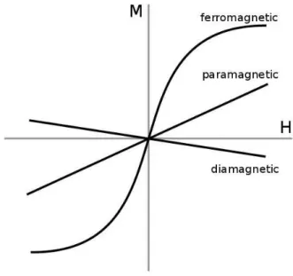
The susceptibility is an important factor for the classiﬁcation of the magnetic materials.

This dimensionless coeﬃcient can be positive or negative, linear or non-linear. The magnetic materials are usually classiﬁed in three main groups: diamagnets, paramagnets and ferromagnets.

Diamagnetic materials contain only atoms and molecules which have no net magnetic moment. In the presence of an applied field, their induced magnetization is weak and opposite to the field direction. The susceptibility values are negative, usually in the range of −10⁻⁶ to −10⁻⁴ and don’t vary with temperature. Diamagnetism is present in all materials, even those containing other types of magnetic materials. Its effects are much weaker than the others and are often negligible. Some common diamagnetic materials used in microsystems are water (χ = −9.06× 10⁻⁶), silicon (χ = −14.0×10⁻⁶), carbon (χ = −16.0× 10⁻⁶) and copper (χ = −22×10⁻⁶). The most diamagnetic natural material is bismuth (χ =

−175.0×10⁻⁶) which is only defeated by the synthetic hyghly oriented pyrolitic graphite (HOPG) (χ=−450.0×10⁻⁶). These materials are the subject of studies concerning stable and actuated magnetic levitation.

The paramagnetic behaviour appears when atoms have a net magnetic moment, but these moments do not interact with each other and are free to rotate in any direction.

When submitted to an external field, paramagnets have their global moment aligned in the same direction of the field creating a net magnetization, which returns to zero if the field is removed. The magnetization is higher at lower temperatures and decreases as temperature increases. This is due to the thermal agitation of the moments, which tend to be less aligned with the field. The M(H) curve also becomes more linear with increasing temperature.

The values of susceptibility for paramagnets are positive and range from 10⁻⁴ to 10⁻³. The paramagnetic behaviour of a material can be described by Langevin’s equation, which states that the magnetization as a function of the ﬁeld and the temperature is

M =M₀cothx− 1

x with x = µ0m0H

kBT (1.5)

where M0 is the saturation magnetization at 0 K, m0 is the modulus of the magnetic moment, kB is Boltzmann’s constant and T is the temperature.

(21)

Ferromagnets, as paramagnets, have a net atomic magnetic moment, but unlike the latter, these moments are strongly coupled together. These coupled moments are spontaneously aligned over large regions called Weiss domains. The temperature, in ferromagnets, also reduces the magnetization by thermal agitation of the moments.

Ferromagnets, despite of the spontaneous magnetization, can have a zero global magnetization. In this case, each domain is randomly aligned, with no preferential direction.

Submitting the material to an increasing magnetic field will align the moments in the same direction, until it reaches saturation. At this point, even if the field is removed, the material will show a global moment due to the preferential orientation of the individual moments. If a field is applied in the opposite direction until saturation and again in the first direction, the magnetization as a function of the field does not follow the same path. This is called hysteresis and is what gives magnets so many potential applications. These loops will be further discussed in section 1.1.3.

Ferromagnets are also characterized by their Curie temperature TC, the temperature at which thermal agitation overcomes the coupling interactions and the material loses its speciﬁc magnetic characteristics. The susceptibility of ferromagnets usually ranges from 10⁴ to 10⁵.

Figure1.1 shows characteristic magnetization curves of diamagnetic, paramagnetic and ferromagnetic materials.

Figure 1.1: Magnetization curves of diamagnetic, paramagnetic and ferromagnetic materials.

1.1.3 Hard and soft magnets

The terms hard and soft magnets come from the analysis of the hysteresis loops of the magnetic materials. Let us, ﬁrst, properly analyse the magnetic structure of ferromagnets

(22)

and their dependance to an applied field. Take a demagnetized ferromagnetic material divided into several randomly oriented Weiss domains. The domains are created to minimize the energy in the material and are affected by defects, inclusions and dislocations. The interfaces between the domains are zones of magnetization reorientation, i.e., transition zones where the moments gradually change from one direction to the other. Felix Bloch, a Swiss physicist, was the first to study the properties of these zones, hence the name Bloch walls. The domain walls have an associated energy and can respond to an applied field.

Consider the material shown in Figure 1.2, initially dividided in a few domains. An applied field induces a torque on the magnetic moments that tends to force them towards the field direction. The Bloch walls are displaced and the domains which are parallel to the field grow, while the other domains are consumed. Saturation is obtained when all the moments are aligned with the magnetic field.

Figure 1.2: Domain walls being displaced by a magnetic field. The increasing magnetic field is represented by the gray arrow.

The saturation state is obtained while the field is being applied. Removing the field causes the magnetization to reduce. In ferromagnets not all the moments reorient after the saturation field is removed. The magnetization remaining at zero field is called remanent magnetization (MR).

The field which is necessary to induce a zero global magnetization on the previously saturated material is called the coercive field HC. At this point the domains are aligned with preferential directions and the sum of the moments results in zero magnetization. Hard and soft magnets are characterized by, respectively, high and low coercivities. The μ⁰HC

values¹ are usually between 0.5 and 2 T for the first and around 10⁻⁵ T for the latter.

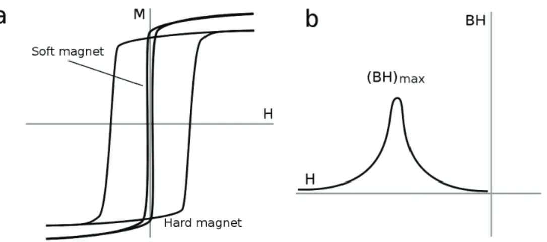
Remanence and coercivity are very important extrinsic properties to observe when looking for high-quality magnets. Varying a field between positive and negative values and observing the consequent magnetization or induction generates the hysteresis loops, so appreciated by magneticians. The so-called M-of-H (M(H)) or B-of-H (B(H)) plots present basically three main quantitative information: the already mentioned MR (or BR, the conversion between the two of them is obtained from equation1.2, the coercive fieldHC

and the energy product (BH)max. The hysteresis loop is completed by going to the negative

1Field and magnetization values are often multiplied by the vacuum permeability and, thus, represented byµ0H andµ0M. The advantage is that the unit becomes the Tesla [T], which is easier to handle.

(23)

Magnet μ⁰MR[T] μ⁰HC[T] BHmax,th[kJ/m³] TC[K]

NdFeB 0.7-1.3 1.0-2.8 514 585

SmCo 0.8 1.0-3.5 220 1000

FePt 0.7 1.0 407 750

AlNiCo 1.2 0.1 44 1200

Ferrites 0.4 0.3 29 720

Table 1.1: Magnets

and back to the positive saturation fields. Figure1.3a shows typical hysteresis loops for hard and soft materials.

Figure 1.3: (a) Typical hysteresis loops for hard and soft magnets. (b) BH(H) curve showing the highest BH product.

The energy product is calculated from the demagnetization curve, which is the portion of the hysteresis loop in the second quadrant. A plot ofBH(H) (Figure 1.3b) allows one to identify the point of maximum product, or (BH)max. This product gives an idea of the energy a magnet can store. Table 1.1 presents the properties of a few commonly used permanent magnets. (BH)max,th represents the theoretical maximum energy product obtained for each magnetic material.

1.1.4 Magnetic particles and the superparamagnetism

Micro- and nanoparticles are used in several domains, from industrial applications to scientific research. Their high surface-to-volume ratio renders these particles especially interesting for the biomedical field. For instance, reducing the radius of a spherical object from 1 mm to 1μm yields an increase in surface by a factor 10⁶ while its volume reduces by

(24)

a factor of 10⁹. In other words, the surface-to-volume ratio increases by 1000 for a reduction of 1000 in the radius of the object.

The interest of the large available surface with low volume is that speciﬁc functional components can be attached to the surface of the particles, allowing their use for labelling, targeting and separation. Yet, the magnetic character of the particles hugely expand their applicability, since remote actuation becomes possible. Nowadays such particles are commonly used for Magnetic Resonance Imaging (MRI)[2, 3], drug delivery [4, 5], hyperthermia [6, 7] and several other applications where a magnetically activated motion can be used. A very important research ﬁeld and application of magnetic particles is now the High Gradient Magnetic Separation (HGMS), in which objects labeled with these particles are sorted due to magnetic actuation. Non-magnetic (or diamagnetic) particles can also be submitted to a magnetic force, as mentioned before.

Magnetic particles are usually considered to be spherically-shaped objects. Their dimension varies from a few nanometres to several micrometres and the size distribution can be very narrow, depending on the fabrication technique. Usually these particles have a polymeric matrix (polystyrene (PS) or latex) - silicon and silicon oxide are also used - and the magnetic character comes from magnetic materials embedded in it (inclusions). The distribution of the inclusions can follow three main structures. Particles in the nanometre range are usually composed by a magnetic core, which is surrounded by a protective, non-magnetic matrix (see Fig. 1.4a). As the size increases, it becomes more recurrent to see the structure of Fig. 1.4b, with many magnetic inclusions in a spherical non-magnetic matrix. A non-magnetic core surrounded by magnetic inclusions and the whole covered by a protective layer (Fig. 1.4c) is more rarely used[8,9].

Figure 1.4: (a) Magnetic core, (b) multiple magnetic cores, (c) magnetic particles surrounding a polymeric core.

The shell which protects the inclusions from the environment is often prepared in such a way that a further functional layer can be attached to the particle. This cover layer is usually biological or chemical and is responsible for the interactions of the particles to speciﬁc targets, which vary from nano (radioactive atoms, biological molecules, DNA chains) to micro-objects (bacteria, cells). Diﬀerent particle fabrication and functionalization techniques are available.

If more information about it is required, it can be found in the following references: [8], [10].

(25)

As regards the magnetic materials incorporated to the particles, the most common are iron and iron oxide - magnetite (F e3O4) and maghemite (γ-F e2O3). These materials are interesting for their magnetization due to the magnetic moment of iron, which is the highest among the ferromagnetic transition metals. Nevertheless, iron is very susceptible to oxidation, thus a protective layer is also required for iron particles. This layer can also serve to render iron and iron oxide magnetic particles biocompatible.

Superparamagnetic particles are preferred for many applications due to some very interesting properties: high susceptibility and absence of remanent magnetization, which could lead to agglomeration under certain conditions. Superparamagnetism appears in ferromagnetic materials when the grain size is reduced down to a few nanometers (1 - 50 nm, depending on the material). Below this dimensional threshold the material presents a behavior which is similar to paramagnetism. An applied ﬁeld can orient the grains in any direction and the removal of this ﬁeld does not leave a remanent magnetization.

The susceptibility of superparamagnetic materials is, however, much larger than that of paramagnetic materials.

The superparamagnetic behavior occurs due to the inﬂuence of temperature on the magnetization when the grain size is smaller than a critical magnetic domain size. The thermal energy induces a random switch of magnetization direction of the small particles.

The magnetic anisotropy of most particles induces, usually, two stable orientations. The average time between two orientation switches is calledNéel relaxation timeTN and depends exponentially on the volume of the particle. Obviously, large grains can have a TN of years and are not superparamagnetic. In the case of the nanometric grains this time is typically in the nanosecond range.

For iron oxide at room temperature the limit in dimension for a particle to become superparamagnetic is around 40 nm [11]. The comercial superparamagnetic microparticles are usually composed by many superparamagneticnanoinclusions embedded in a micrometric matrix.

The superparamagnetic behaviour can also be modeled by the Langevin function (equation1.5). This behaviour is characterized by a high susceptibility at low magnetic ﬁelds, followed by saturation at a few hundreds ofmT. As previously mentioned, the magnetization of a superparamagnetic material returns to zero when the ﬁeld is removed, as observed in Figure 1.5. A more detailed model of the particle magnetization is given in Chapter 4.

(26)

Figure 1.5: Typical magnetization curve for a superparamagnetic material.

Magnetism and magnetic particles become even more interesting for a number of applications when coupled to microﬂuidics. The possibility to act on the ﬂow of a liquid solution while acting on the particles themselves render magnetic labeling a major technique, for instance, for the study of bacteriologic processes and cell sorting.

1.2 Microfluidics

One of the most simple and precise descriptions of what microfluidic is was given by Whitesides in 2006: “It is the science and technology of systems that process or manipulate small amounts of fluids (10⁻⁹ to 10⁻⁸ litres), using channels with dimensions of tens to hundreds of micrometres” [1]. In this same Nature paper Whitesides mentions that, despite of the many advantages it offers, microfluidics is not widely used. It rapidly changed in the following years, as indicates ISI Web of Knowledge: around 100 papers citing microfluidics in 2000 against more than 3000 papers in 2010. Today microfluidics is widely spread and its applications go from simple channels to very complex systems integrating electrical, mechanical, and optical parts.

What makes microﬂuidics so interesting are its fundamental characteristics, which bring many advantages:

• Very small amounts of liquid: very low waste of materials, which is very interesting for precious samples.

• Fast reactions: due to the small volumes, reactions don’t depend on the time-consuming mixing over large distances and can occur in a controlled and fast fashion.

(27)

• Laminar flow: (discussed further in this chapter) a great advantage of the scale reduction. Controlled mixing can be performed or mixing can be easily avoided. The fluid flow can also be easily predicted and modeled.

• Polymer-based devices: microﬂuidics is compatible with several polymer-based technologies, which makes it an easy, fast and cheap alternative to glass or silicon.

Many other advantages - such as the possibility to functionalize the polymeric surfaces of a microfluidic channel and the small environmental footprint of these devices - can be derived from the list above. The list is not exhaustive, as this field is constantly evolving with different materials, fabrication methods and applications.

1.2.1 Scaling laws and the continuum hypothesis

The ﬁrst thing that pops out when analyzing the properties of microsystems is the surface-to-volume force ratio. Surface forces are proportional tol²- wherelis a characteristic dimension of the system - and volume forces are proportional to l³. Analyzing the ratio of these forces yields

l²

l³ =l⁻¹; if l−→0, surf acef orces

volumef orces −→ ∞. (1.6) Put in words, volume forces are usually predominant at the macroscale, while for microﬂuidics, surface force eﬀects and surface interactions are essential.

Microﬂuidic devices are supposed to handlefluids, i.e. liquids or gases. The interactions in a liquid are much more complex, since each molecule is always surrounded by many others. At short ranges the molecules can be considered ordered around determined positions.

Nevertheless, as opposed to solids, in which the thermal oscillations makes atoms move slightly around a precise position in a lattice, the oscillations in liquids make them able to flow. Even though fluids are composed by atoms and molecules, for most applications in microfluidics they can be analyzed as a continuous entity. Thiscontinuum hypothesisrenders much easier the analysis and prediction of fluid properties and dynamics. The hypothesis is valid up to a maximum volume, above which the environment can change the local properties of the fluid, e.g. a force applied on a liquid can locally change its density [12].

1.2.2 Reynolds number and flow regimes

Microscopic fluid flows are typically very different from the day-to-day macroscopic flows (washing your hands in the sink, pouring orange juice in a glass). The reduced dimensions of a microfluidic channel induce a modification in how the fluid behaves: the common turbulent regime becomes in this case a smooth laminar regime. These regimes are characterized by a distinct Reynolds number, which is simply a relation between inertial and the viscosity forces.

(28)

The dimensionless Reynolds number comes from an analysis of the Navier-Stokes equation, represented below, which describes the evolution of a velocity vector ﬁeld. Velocity is represented~u,t is the time, ρand µare the density and the viscosity of the ﬂuid and pis the pressure.

∂~u

∂t + (~u· ∇)~u =−1

ρ∇p+µ

ρ∇²~u (1.7)

The viscous and inertial eﬀects can be analyzed by taking a characteristic velocity U and a characteristic length L and scaling the terms of the equation. One can observe that

~u scales with U and t scales with _U^L (advection time scale). It implies that the unsteady inertial term ^∂~_∂tû scales with Û_L². The spatial derivative ∇scales with _L¹, thus, the non-linear inertial term (~u· ∇)~u also scales with Û_L². Finally, the viscous term ^µ_ρ∇²~u scales with _ρL^µU2.

The inertial-to-viscous ratio, i.e. the Reynolds number is, thus, given by:

Re= ulρ

µ . (1.8)

A turbulent regime occurs typically when the Reynolds number is higher than 4000.

In this case the inertial forces are predominant and the flow is characterized by a chaotic movement of the fluid. The mean velocity is “forward”, so the water comes out from the hose and you can water your garden, but inside the hose the water streamlines are going in every direction permanently. Figure 1.6a schematically shows how a fluid flows inside a channel in a turbulent regime.

If the size of the channel is suﬃciently reduced, the laminar regime is achieved (Re <

2300). In this case the streamlines become organized and regular, as shown in Fig. 1.6b. This type of flow regime can be compared to a set of playing cards piled up on a table. Tilting the table makes the cards slide above each other with different velocity, but they remain parallel as they move. In other words, the fluid particle follows a determined streamline along the channel and is not constantly mixed with the neighbouring fluid particles.

Below 4000 and down to around 2000 the flow regime is characterized by a transient state, which is both turbulent and laminar. Viscous and inertial effects occur concurrently, the first more concentrated around the edges of the pipe or tube, and the latter on the zones not affected by the boundary effects.

(29)

Figure 1.6: (a) Turbulent flow. (b) Laminar flow.

Typical microfluidic devices induce Reynolds numbers around 1, frequently even less. It means that going to the micron scale rapidly reduces the mass on the system, thus reducing inertial effects. On the other hand, surface and viscous effects quickly become important.

The result is a very smooth, predictable laminar flow inside the microfluidic channels.

The parabolic velocity profile observed in laminar regimes comes from the effect of the edges of the channel on the flowing fluid. In a turbulent regime the effect of theboundary layer does not “penetrate’ on the fluid significantly. Inversely, the boundary layer progressively penetrates on a laminar flow, resulting in a modification of the velocity profile seen in Figure 1.7. Once the effects of all the edges of the channel are stable, a continuous parabolic profile is observed.

Figure 1.7: Influence of the boundary layer on the fluid flow.

Turbulent regimes present a few advantages, such as the possibility of mixing liquids at high speed and homogeneously, while in laminar regime one has to count on interdiffusion between the liquids - which is often a very slow process - or on adapted microchannels in which vortices or perturbed streamlines are present. Nevertheless, the laminar regime has a major advantage, possibly the one responsible for its succes among microdevices:

predictability. Laminar flows can be described mathematically and simulated with very high precision. In this manner, microfluidic devices are modeled and optimized before being fabricated. Controlled chemical reactions, interdiffusion of liquids and the trajectory of particles can be precisely predicted, even in devices integrating multiple techniques, i.e.

microfluidics, electricity, magnetism. [13]

(30)

1.2.3 Digital and continuous flow microfluidics

Two main techniques of fluid manipulation are used in microfluidic devices. The first one, called digital microfluidics, is used to manipulate isolated amounts of fluid, ordroplets. The advantages brought by this technique are the significant reduction in the required sample volume and the possibility of analyzing many samples at once. Precise amounts of liquid can react with each other and be observed at high speed. However, this technique often requires a complex apparatus.

The second technique, continuous flow microfluidics, is the most widespread today.

It consists simply on passing the fluid continuously through the microchannel. The fluid displacement is induced, in most cases, by a difference in pressure between the inlet(s) and the outlet(s) of the channel. Apart from this pressure-driven flow, other two common methods are theelectrokinetic flow, where the fluid flows due to an applied electric field, and the capillary flow, where capillary forces induce the movement. This last method has the drawback of only working with very low channel dimensions and while the channel is not completely wet, but also the advantage of handling very small amounts of liquid.

Pressure-driven ﬂow is used for all the systems used in this research. The diﬀerence in pressure is achieved mostly by applying a higher pressure on the inlets of the channel.

However, for certain applications, a lower pressure is applied on the outlets (the liquid is pumped out).

1.2.4 Flow cytometry

Flow cytometry appears in a significant part of scientific papers dealing with micro-object handling, as it can be seen in the context overview of Section1.3. This technique is today very reliable for counting and separating objects in the microscale at a very high speed. It is used in several domains, mainly in cell biology and medicine. The equipment required to perform flow cytometry is complex and expensive, but the principle can be simplified as presented below.

The ﬁrst important point to notice is that ﬂow cytometry - cyto comes from the greek and stands for cell or hollow, but is mainly used for animal or plant cells - is not only used to sort cells. It can be used with molecules, particles and other objects in liquid solution.

In fact, ﬂow cytometry is not used only to sort these objects. Some ﬂow cytometers are not even capable of performing sorting, in spite of the wide use of the name FACS (which is an acronym for Fluorescence Activated Cell Sorting and, actually, a trademark). This technique is sometimes used simply to count distinct populations of objects in a same solution. [14].

A ﬂow cytometer is composed by three main parts:

1. A source of focused light, usually a laser;

2. A ﬂuidic system capable of aligning the objects of study in a stream;

3. An electronic part to collect and analyze the signals.

(31)

The basic scheme is shown in Figure 1.8. The liquid solution containing the objects of interest passes through the fluidic system of the equipment and is focused in a single stream.

The goal is to obtain a stream sufficiently thin so that the objects flow separately. In a basic configuration, a laser irradiates the objects and is blocked/diffracted in a characteristic fashion depending on the object’s content and properties. Two signals are collected: the transmitted beam at low angles (0.5 - 10^◦) from the axis (forward scattered, FSC) and the refracted beam at 90^◦ (side-scattered, SSC). The FSC beam gives the object radius. The second beam is scattered due to the inhomogeneities of the object (the nucleus of a cell or inclusions in a latex particle), so it gives an idea of the content of the object. Some flow cytometers are equipped with multiple laser sources which are used to excite specific fluorescent groups tagging the objects. The electronic part is responsible for collecting these signals and transmitting them to the analyzer.

Figure 1.8: Schematic of the flow cytometry principle.

Flow cytometers work in a multiparameter fashion, i.e., all the informations - size, granularity, fluorescence - are collected for each object. It facilitates the discrimination of several populations when some parameters are similar. Consider, for instance, two populations of cells in a solution, one population is tagged with fluorescent magnetic nanoparticles, while the other is not modified. Analyzing FSC×SSC plots for these populations may result in superimposed groups of data, since the size and the granularity

(32)

are not so different (see Figure 1.9a). Plotting the fluorescent signal versus the granularity (Fig. 1.9b) or versus the size (Fig. 1.9c) will result in two very distinct populations, since the non-tagged group shows no fluorescence signal, while the signal for the tagged group is very strong.

Figure 1.9: Two groups of objects analyzed by flow cytometry. The groups are superimposed in the (a) FSC×SSC plot, but can be better discriminated if one of them is tagged with a fluorescent agent (FITC), as shown in (b) the FSC×FITC plot and (c) the SSC×FITC plot.

The treatment and analysis of the data is often complex, due to overlapping of fluorescence spectra and the need of compensation factors. In the case of FACS equipments (those actually performing sorting), the liquid stream is turned into separate drops of liquid, which are then electrically charged in order to be deviated by charged plates and collected into different recipients.

1.3 State of the art: handling micro-objects

As mentioned in the introduction of this chapter, not only magnetophoresis is used to handle objects at the micron scale. Other forces coming, for instance, from sources as simple as the perturbations on the streamlines of a microfluidic flow caused by the channel structure itself are used.

Hydrodynamic effects can be used to change particle trajectory in a microfluidic channel.

This is maybe the simplest actuation technique, since it can be based only on the shape of the channel. The perturbations on the streamlines caused by the shape of the channel are responsible for the force acting on the particles. Di Carlo et al. developed a micro-channel configuration which allows particles to be focused on its center due to these effects [15].

The particles enter the channel randomly dispersed and, as they move through the curves of the channel, are focused both longitudinally and laterally, i.e. one single line of particles is obtained (see Fig. 1.10a). The group attributes particle focusing to lift forces in the cases where inertial effects are significant.

Similarly, but in a more controllable, yet more complex fashion, Wang et al. [16]

(33)

developed a system which deviated the trajectory of a particle by a change in the fluid flow. A piezoeletric transducer coupled to the micro-channel is responsible for the control of a bubble produced on the edge of the channel (see Fig. 1.10b). Changing the size of the bubble induces a modification in the streamlines around it, thus deviating a particle in its vicinities. Particle separation is demonstrated with high precision using this system.

Figure 1.10: (a) Particle focusing using hydrodynamic forces [15]. (b) Particle deviation by a modiﬁcation in the streamlines caused by bubble controllable in size[16].

Acoustic forces are also an option for contactless actuation. Considering the case of acoustic actuation with microfluidics, the basic principle is to generate standing sound waves in the channel. These waves can be produced in such a way that nodes and anti-nodes are generated at different points of the channel. Once an object enters the channel a radiation force acts on it, pushing it to a node or an anti-node, depending on various factors (acoustic properties of the object, its density and compressibility, etc.). This radiation force is actually a sum of two forces: a primary force coming from the standing wave and a secondary force - orders of magnitude smaller and only significative at small distances - coming from the sound waves scattered by the object [17].

Adams et al. used this technique to sort particles of different sizes [18]. In this paper the group reports on the separation of three sizes of particles, using the system shown in Figure 1.11a. The particles enter the microfluidic channel by its extremities, while a buffer solution is inserted at the center. The first separation occurs in the beginning of the channel, where the whole solution is submitted to an acoustic radiation force. Different responses to the force are presented by each type of particle. The acoustic forces focuses two groups of particles in the center of the channel, while the third group is slightly deviated and collected in the low-pass outlets. The deviated particles are then guided to the extremities of the channel,

(34)

a buﬀer solution being inserted in the center, and submitted to a second acoustic radiation force, which is diﬀerent in this stage and focuses only one group of particles in the center of the channel. Outlets conveniently disposed in the end of the channel collect each group of particles. Adams et al. also used acoustophoretic forces combined with magnetophoretic forces to separate three types of particles in another system, reported in [19].

Figure 1.11: Acoustic forces used to sort (a) microparticles [18] and (b) reb and white blood cells [20].

Another work developed by Petersson et al. used acoustic forces to separate red blood cells from lipid particles in whole blood [20]. In this case, the acoustic radiation force concentrated the red blood cells on the nodes of a standing acoustic wave, while the lipids were guided to the anti-nodes of the wave. A schematic of the separation mechanism is reproduced in Fig. 1.11b. The objects were then collected by three outlets in the end of the microchannel.

Dielectrophoretic (DEP) forces are also widely used for continuous flow sorting. In dielectrophoresis and uncharged object can be displaced due to a force generated by an electric field gradient. This external field will polarize the dielectric material, which will have, thus, an internal electric field. The internal field can be represented by a dipole which is aligned with the external field at a point. As the object moves in the field gradient, a force acts on it, deviating its trajectory [21].

(35)

Kim et al. reported on the use of this force for the separation of mammalian cells [22].

The system so used contains a ﬁrst set of electrodes which focus the cells at a certain point of the channel and a second set which deviates the cells according to their size, as shown in Figure 1.12a. With this technique, cells in diﬀerent cycle phase could be sorted, since to each phase corresponds a cell dimension.

Figure 1.12: (a) Particle focusing and deviation using dielectrophoresis [22]. (b) Sorting of particles based on the dielectric character [23].

Han et al. used dielectrophoresis to perform separation of red and white blood cells [24].

In this work separation occurs due to a diﬀerence of sign in the force acting on each type of cell resulting in simultaneous positive and negative DEP.

In another work [23], the group reports on the separation of blood cells according to their size, using the same type of actuation. Figure1.12b, adapted from Han’s article, shows a microfluidic channel with two sets of electrodes aligned with a certain angle related to the fluid flow. Blood cells are differently deviated by the electrodes and can be collected in independent outlets further in the channel. The DEP force becomes stronger as the cell size increases.

The optical force created by a light source - a laser, for instance - can also be used to

(36)

deviate objects. Both angular and linear momenta can be transferred to a micro-particle, for instance, when the latter is irradiated. [25]. This optical force can be separated into two components: the gradient force (or dipole force) and the scattering force. These work both with micro and nano-particles and can be computed, as shown by Rohrbach and Stelzer in [26,27], if the particle size is signiﬁcantly diﬀerent to the wavelength of the irradiating light.

Wang et al. reported on the separation of mammalian cells in microﬂuidic channel using optical switching in [28]. Particle deviation was reported later on by Hoi et al. [29]. Their technique consists of ﬂowing the micro-particles through a channel, and acting on them by means of a laser beam which is focused at a certain point inside the channel. As it can be observed in Figure 1.13, the particles can be deviated towards an outlet which is positioned at a certain angle related to the main channel. The amount of deviated particles can be adjusted by controlling the angle of incidence of the laser.

Figure 1.13: Control of particle trajectory using optical forces [29].

1.3.1 Magnetic flux sources

As previsouly discussed, three types of magnetic ﬂux sources are used to perform magnetophoresis (MAP) of micro and nano-objects: permanent magnets, electromagnets and soft magnets. In this section an overview of recent publications on magnetophoresis using these three methods is given. It is not an exhaustive overview, for it intends simply to give an idea of materials and methods used nowadays (in particular MAP coupled to microﬂuidics) and for this research domain is constantly evolving.

Permanent magnets at the macro and at the micro-scale are treated here as two different types of magnetic flux sources. One can deduce that the physics behind both of them is the same, which is right. The discrimination here has two purposes: to stress that the constraints in fabrication methods for these two types of magnets are very different; and to emphasize that great advantages of permanent magnets for micro-object handling are only observable with magnets at the micro-scale.

(37)

Bulk permanent magnets

Permanent magnets at the macro-scale (bulk) were the first sources of magnetic field to be combined to microfluidic channels in order to attract magnetic particles. The ease to produce such sources of field in different shapes and sizes and to integrate them to the devices, combined with the high magnetic field created by the rare-earth permanent magnets, was decisive for their success on the field of magnetic separation.

As it will be discussed in Chapter 4, in order to generate a significant magnetic force on an object, both high magnetic field and field gradient are required. Bulk magnets generate intense fields at a large distance, compared to the µm- or mm-sized fluidic channels. Their highest magnetic field gradients, however, are restricted to the edges of the magnet, and are often not so consequent inside the microfluidic channel, depending on magnet-channel configuration.

Soft magnets

Soft magnets are one of the most developed domains for HGMS. Basically, the soft magnets used for MEMS are the materials which show a significant magnetization only when polarized by an external magnetic field. In the absence of the polarizing field, these materials create