HAL Id: tel-00763369
https://tel.archives-ouvertes.fr/tel-00763369
Submitted on 10 Dec 2012
HAL is a multi-disciplinary open access archive for the deposit and dissemination of sci- entific research documents, whether they are pub- lished or not. The documents may come from teaching and research institutions in France or abroad, or from public or private research centers.
L’archive ouverte pluridisciplinaire HAL, est destinée au dépôt et à la diffusion de documents scientifiques de niveau recherche, publiés ou non, émanant des établissements d’enseignement et de recherche français ou étrangers, des laboratoires publics ou privés.
l’inférence conditionnelle et aux méthodes d’Importance Sampling.
Virgile Caron
To cite this version:
Virgile Caron. Un théorème limite conditionnel. Applications à l’inférence conditionnelle et aux méthodes d’Importance Sampling.. Statistiques [math.ST]. Université Pierre et Marie Curie - Paris VI, 2012. Français. �NNT : �. �tel-00763369�
École Doctorale de sciences mathématiques de Paris Centre
Thèse de doctorat
Spécialité : Mathématiques Option : Statistique
présentée par
Virgile Caron
Un théorème limite conditionnel.
Applications à l’inférence conditionnelle et aux méthodes d’Importance Sampling.
sous la direction du Professeur : MICHEL BRONIATOWSKI
Soutenue le 16 Octobre 2012 devant le jury composé de :
M. Eric MOULINES Télécom ParisTech président
M. François LE GLAND INRIA Rennes rapporteur
M. Christian P. ROBERT Université Paris Dauphine rapporteur
M. Gérard BIAU Université Paris VI examinateur
M. Gilles PAGES Université Paris VI examinateur
M. Michel BRONIATOWSKI Université Paris VI directeur
3
Laboratoire de Statistique Théorique et Appliquée (LSTA)
Université Pierre et Marie Curie - Paris 6
Tour 15-25, 2ème étage 4 place Jussieu
75252 Paris cedex 05
École doctorale de sciences mathéma- tiques de Paris centre Case 188
4 place Jussieu 75 252 Paris cedex 05
Remerciements
Au moment où s’achève ma thèse, je tiens à exprimer ma profonde reconnaissance à Michel Broniatowski, qui l’a dirigée. Ce fut un grand privilège d’apprendre avec lui et je le remercie vivement pour ses conseils avisés, sa rigueur scientifique, sa disponibilité et son soutien bienveillant.
François Le Gland et Christian Robert ont accepté d’être les rapporteurs de ce travail.
J’imagine le travail que représente la lecture d’une thèse et les en remercie sincèrement.
J’adresse mes sincères remerciements à Monsieur Eric Moulines d’avoir accepté de présider mon jury de thèse, à Messieurs Gérard Biau et Gilles Pagès pour l’intérêt qu’ils ont accordé à mon travail et pour avoir accepté de participer au jury.
J’adresse également mes remerciements à Paul Deheuvels, directeur du LSTA, pour m’avoir accueilli dans ce laboratoire au sein duquel j’ai disposé de conditions idéales pour écrire cette thèse.
Un grand merci à toute l’équipe administrative du laboratoire, Louise Lamart, Anne Durrande et Corinne Van Lieberghe pour leur gentillesse et leurs compétences. Parce que la recherche en mathématiques ne se conçoit pas sans bibliothèque, merci à Pascal Epron.
L’ambiance chaleureuse et la solidarité de l’équipe des doctorants du LSTA ont été importantes pour moi au cours de cette thèse. Merci à Zhansheng, Sarah, Manu, Olivier, Assia. Un grand merci aussi à tous les doctorants qui ont refusé de me donner cinq euros pour voir leur nom apparaître ici. Merci à tous mes amis pour leurs encouragements et tous ces bons moments partagés. Enfin, je voulais remercier ma famille qui a toujours cru en moi. Leur soutien permanent et irremplaçable m’a permis de surmonter les moments difficiles.
Pour finir, je remercie ma femme Emilie, l’amour de ma vie, qui a été à mes côtés durant toutes ces années. 1052019135
Résumé
Cette thèse présente une approximation fine de la densité de longues sous-suites d’une marche aléatoire conditionnée par la valeur de son extrémité, ou par une moyenne d’une fonction de ses incréments, lorsque sa taille tend vers l’infini. Dans le domaine d’un condi- tionnement de type grande déviation, ce résultat généralise le principe conditionnel de Gibbs au sens où il décrit les sous suites de la marche aléatoire, et non son comporte- ment marginal. Une approximation est aussi obtenue lorsque l’événement conditionnant énonce que la valeur terminale de la marche aléatoire appartient à un ensemble mince, ou gros, d’intérieur non vide. Les approximations proposées ont lieu soit en probabilité sous la loi conditionnelle, soit en distance de la variation totale. Deux applications sont développées ; la première porte sur l’estimation de probabilités de certains événements rares par une nouvelle technique d’échantillonnage d’importance ; ce cas correspond à un conditionnement de type grande déviation. Une seconde application explore des méthodes constructives d’amélioration d’estimateurs dans l’esprit du théorème de Rao-Blackwell, et d’inférence conditionnelle sous paramètre de nuisance ; l’événement conditionnant est alors dans la gamme du théorème de la limite centrale. On traite en détail du choix effectif de la longueur maximale de la sous suite pour laquelle une erreur relative maximale fixée est atteinte par l’approximation ; des algorithmes explicites permettent la mise en oeuvre effective de cette approximation et de ses conséquences.
Mots-clefs
Principe de Gibbs ; marche aléatoire conditionnée ; grande déviation ; moyenne dévia- tion ; Importance sampling ; inférence conditionnelle ; Théorème de Rao-Blackwell ; familles exponentielles ; paramètre de nuisance.
Abstract
This thesis presents a sharp approximation of the density of long runs of a random walk conditioned on its end value or by an average of a functions of its summands as their number tends to infinity. In the large deviation range of the conditioning event it extends the Gibbs conditional principle in the sense that it provides a description of the distribution of the random walk on long subsequences. An extension for the approximation of the conditional density in the multivariate case is provided. Approximation of the density of the runs is also obtained when the conditioning event states that the end value of the random walk belongs to a thin or a thick set with non void interior. The approximations hold either in probability under the conditional distribution of the random walk, or in total variation norm between measures. Application of the approximation scheme to the evaluation of rare event probabilities through Importance Sampling is provided. When the conditioning event is in the zone of the central limit theorem it provides a tool for statistical inference in the sense that it produces an effective way to implement the Rao- Blackwell theorem for the improvement of estimators; it also leads to conditional inference procedures in models with nuisance parameters. An algorithm for the simulation of such long runs is presented, together with an algorithm determining the maximal length for which the approximation is valid up to a prescribed accuracy.
Keywords
Gibbs principle; conditioned random walk; large deviation; moderate deviation; simu- lation; Importance sampling; conditional inference; Rao-Blackwell Theorem; exponential families; nuisance parameter.
Table des matières
Introduction 11
1 Long runs under a conditional limit distribution. 17
1.1 Context and scope . . . 17
1.2 Random walks conditioned on their sum . . . 19
1.3 Random walks conditioned by a function of their summands . . . 25
1.4 Conditioning on large sets . . . 40
1.5 Appendix . . . 45
2 Towards zero variance estimators for rare events probabilities 59 2.1 Introduction. . . 59
2.2 Adaptive IS Estimator for rare event probability . . . 61
2.3 Compared efficiencies of IS estimators . . . 62
2.4 Algorithms . . . 68
2.5 Simulation results . . . 69
2.6 A comparison study . . . 70
3 Conditional inference in parametric models. 77 3.1 Introduction and context. . . 77
3.2 The approximate conditional density of the sample . . . 78
3.3 Sufficient statistics and approximated conditional density . . . 82
3.4 Exponential models with nuisance parameters . . . 86
4 Extension au cas d-dimensionnel 93 4.1 Introduction. . . 93
4.2 Hypothèses et Notations . . . 93
4.3 Marche aléatoired-dimensionnelle conditionnée par sa somme. . . 98
4.4 Extension à un cas plus général de conditionnement . . . 102
4.5 Comment choisir k ? . . . 104
4.6 Exemples de Trajectoires dans un cas simple . . . 106
4.7 Familles exponentielles courbes et conditionnement. . . 110
4.8 Démonstration du Théorème 1 du Chapitre 4. . . 118
A Exemples de simulation 137 A.1 Loi Normale. . . 137
A.2 Loi Gamma . . . 139
A.3 Loi Weibull . . . 141
A.4 Loi de Gumbel . . . 141
A.5 Loi Inverse-Gaussienne . . . 141
Bibliographie 143
Introduction
Cette thèse présente un résultat de nature probabiliste, en lien avec le principe condi- tionnel de Gibbs, et deux applications. La première est liée à l’évaluation numérique de probabilités d’événements rares. La seconde est de nature directement statistique et ex- plore des méthodes constructives d’amélioration d’estimateurs dans l’esprit du théorème de Rao-Blackwell, et d’inférence conditionnelle sous paramètre de nuisance, dans la lignée des travaux de l’école danoise.
Approximations de lois conditionnelles
NotonsXn1 = (X1, ...,Xn),ncopies i.i.d. d’une variable aléatoireX de densitépet de loiP surRetS1,nleur somme,S1,n:=X1+...+Xn.On considère une contrainte surS1,n de la forme (S1,n=nan) où la suite an est supposée convergente. Pour k = kn < n, on s’intéresse à la densité du vecteurXk1 = (X1, ...,Xk) sous la contrainte locale (S1,n =nan) pour divers choix de la suitean et de la taillekndu vecteurXk1.Ensuite nous considérons des contraintes globales de la forme (S1,n ∈nA) où A est un ensemble borélien de R d’intérieur non vide. Les contraintes sont ensuite remplacées par des conditions de la forme (U1,n=nan) et (U1,n ∈nA) oùU1,n :=u(X1) +...+u(Xn) et uest une fonction à valeurs réelles telle queu(X1) admette une densité. Enfin, on considère le cas où lesXi sont des vecteurs aléatoires de Rd et on s’intéresse à la densité du vecteur Xk1 sous une contrainte locale.
Cette classe de problèmes conditionnels limites porte le nom deprincipes conditionnels de Gibbs et trouve sa source dans l’étude de systèmes thermodynamiques développée à la fin du 19ème siècle et au début du 20ème siècle par Boltzmann, puis par Gibbs, sous le nom de lois microcanoniques lorsque k = 1. Des approches directement probabilistes ont été développées dans les années 1970 en lien avec la théorie des grandes déviations, et développées, entre autres, dans le cadre du théorème de Sanov par [26], et par de nombreux auteurs.
Le contexte de notre étude est caractérisé par le fait que la longueurk du vecteurXk1 peut être très grande, puisque nous imposons les conditions
0≤lim sup
n→∞k/n≤1 (K1)
et
n→∞lim n−k=∞. (K2)
La suiteanest supposée converger soit versEX1(resp. versEu(X1)) ou vers une valeur différente. Ce second cas est définit une contrainte locale de type "grande déviation" ; le premier cas peut correspondre à plusieurs situations distinctes : moyenne déviation si
√n(an−Eu(X1)) → ∞ , ou relevant du domaine du théorème de la limite centrale si
√n(an−Eu(X1)) = 0(1).
Contexte bibliographique succint
Quandk est indépendant den(typiquement k= 1), les résultats que nous présentons sont des généralisations duPrincipe Conditionnel de Gibbs qui a été étudiée pouran fixé, différent deEX1, sous une condition de grande déviation. Diaconis et Freedman [33] ont considéré ce problème dans un cas un peu plus général,k/n→θ pour 0≤θ <1, en lien avec le théorème de de Finetti pour des suites finies échangeables (voir [88] pour détails).
Leur intérêt est lié à l’approximation de la densité deXk1 par le produit des densités des variables aléatoiresXi, c’est à dire à la permanence de l’indépendance asymptotique sous le conditionnement local de la somme des variables.
Leur résultat, dans l’esprit de [93], est à mettre en parallèle avec le travail de [26]
sur l’indépendance conditionnelle asymptotique lorsque l’événement conditionnant est (S1,n> na) où a > EX.Dembo et Zeitouni [29] considèrent des problèmes semblables.
En physique statistique, de nombreux articles se rapportant aux propriétés structurelles des polymères traitent de l’approximation de la densité conditionnelle ; voir [30] et [31].
Dans le cas des moyennes déviations, Ermakov [44] considère aussi un problème similaire pourk= 1.
Le cas d’un conditionnement de type central limite (lorsque√
n(an−Eu(X1)) = 0(1)) a reçu peu d’attention dans la bibliographie liée à l’approximation des lois conditionnelles, puisque asymptotiquement la loi conditionnelle de S1,k est de l’ordre de celle sans condi- tionnement (voir par exemple [94]), lorsquekne dépend pas den. Cependant cette question s’avère d’une grande importance pour l’inférence statistique. Nous indiquons brièvement quelques approches dans ce domaine ; le chapitre 3 présente une bibliographie plus étoffée.
Pedersen [76] approxime la densité conditionnelle, non pas, du vecteur Xk1 mais direc- tement la densité de la statistique de test conditionnellement à une contrainte locale.
L’intégration cette approximation lui permet d’obtenir des valeurs critiques (voir [9] ou [75]). D’autres approches ont été récemment proposées (voir [71], [42], [67] et [68]). Leur but n’est pas d’obtenir une approximation de la densité conditionnelle, mais de développer des algorithmes permettant directement la simulation d’échantillon sous la densité condi- tionnelle. Ces méthodes algorithmiques sont valides sous certains modèles, et non valides sous d’autres. Elles ne permettent pas d’obtenir une méthode unifiée pour les distribu- tions continues les plus courantes. Pour chaque loi étudiée, une nouvelle méthode doit être fabriquée.
Méthodes
Dans son livre "Saddlepoint approximation", Jensen [59] commence son chapitre 1 par la comparaison des trois méthodes les plus classiques pour approximer la densité d’une somme de variables aléatoires indépendantes de même loi :
1. l’approximation résultant de l’utilisation de la densité normale de même espérance et variance que la densité de départ
2. l’utilisation de l’approximation d’Edgeworth améliorant la méthode précédente 3. l’approximation de point selle, qui utilise une famille de lois conjuguées remplaçant
l’approximation normale directe, liée ensuite à l’utilisation de développements d’Ed- geworth.
En comparant sur un exemple ces trois méthodes, il remarque que l’approximation d’Edgeworth améliore la première méthode au mode de la densité seulement, mais pas aux endroits où la densité est faible, alors que l’approximation point selle est bonne par- tout. L’approximation point selle est basée sur la relation entre la densité de départ et
Introduction 13 la densité conjuguée (ou tiltée) qui est obtenue en multipliant la densité de départ par exp (tx), pour un t appartenant au support de P, et en la renormalisant. Ce que Jen- sen nomme "classical saddlepoint approximation" dans son chapitre 2, est une méthode d’approximation effectuée en deux étapes. Il relie, tout d’abord, la densité de départ à sa densité conjuguée, puis il utilise un lemme fondamental, qui énonce la commutativité de la conjugaison et de la convolution ; l’approximation d’Edgeworth est appliquée à la convolution des conjuguées, ce qui fournit finalement l’approximation de la densité de la somme normalisée des variables initiales.
Pour l’obtention de l’approximation de la densité conditionnelle proposée au Chapitre 1, nous appliquons une méthode utilisant des ingrédients semblables. En effet, la démons- tration principale repose sur plusieurs éléments clés en plus de celui dont nous venons d’évoquer. Pour obtenir cette approximation, sont utilisés dans la preuve : la formule de Bayes, un lemme d’invariance sous la densité tiltée et des développements d’Edgeworth ainsi qu’un contrôle précis des caractéristiques des chemins typiques. La méthode de dé- monstration s’applique de façon identique quel que soit le type de conditionnement. Des différences importantes apparaitraient si l’on s’intéressait au cas où an → ∞, hors du contexte de cette thèse.
Amélioration proposée
Le Chapitre 1 présente un théorème d’approximation de la loi conditionnelle d’une longue sous trajectoire. Ce théorème est ensuite travaillé dans divers contextes, menant à des versions diverses. En effet, un changement dans la structure de dépendance des Xi sous le conditionnement, quand (K2) et (K1) sont satisfaites, est exhibé et une so- lution constructive pour le schéma d’approximation est fournie, à l’aide d’algorithmes et d’exemples. La densité approximante est obtenue comme une version légèrement modifiée du tilting classique, combiné à un changement dans la variance. Les résultats améliorent les résultats mentionnés puisque ils procurent une approximation plus fine de la densité conditionnelle même quand k est très proche de n. Le résultat présenté coïncide dans le cas gaussien avec la loi conditionnelle exacte sur toute la trajectoire ; en ce sens le résultat obtenu est optimal. Dans le domaine d’un conditionnement de type grande déviation, ce résultat généralise le principe conditionnel de Gibbs au sens où il décrit les sous suites de la marche aléatoire, et non son comportement marginal.
L’aspect crucial de notre résultat est le suivant. L’approximation de la densité deXk1 conditionnée à (U1,n =nan) n’est pas obtenue surRktout entier, mais plutôt sur une suite de sous-ensemble deRk qui contient les trajectoires simulées sous la densité conditionnelle (de même, pour les trajectoires simulées sous son approximation) avec probabilité ten- dant vers 1 quandn tend vers l’infini. Ainsi, l’approximation est obtenue sur les chemins typiques. Les raisons, pour lesquelles nous considérons l’approximation de cette manière sont de deux sortes.
1. En inférence conditionnelle, l’approximation doit être valide sur les trajectoires simu- lées sous la densité conditionnelle, tandis que, pour des applications en Importance Sampling, elle doit être valide sur les trajectoires simulées sous la densité approxi- mante.
2. Un nombre important de conditions techniques nécessaires pour obtenir une approxi- mation sur tout l’ensembleRk et centrales dans les articles mentionnés ci-dessus est ainsi évité. Ces conditions portent sur la fonction caractéristique de la densité p de X pour obtenir une bonne approximation sur tout Rk. Puisque l’approximation conditionnelle est obtenue uniquement sur les chemins typiques sous la densité condi-
tionnelle deXk1 et sous le conditionnement ponctuel, les régions deRk ainsi atteintes sont mieux connues. Cependant, même sous ces hypothèses plus faibles, un résultat d’approximation sur Rk tout entier est obtenu. En effet, la convergence de l’erreur relative sur les grands ensembles implique que la distance en variation totale entre la loi conditionnelle et son approximation tend vers 0 sur Rk tout entier. Ce résultat généralise ceux de [33] et [29], portant sur le cas oùkest petit devantn. Néanmoins, notre résultat ne procure pas de vitesse de convergence.
Application au calcul de probabilités d’événements rares
Le résultat d’approximation présenté dans le premier chapitre permet, quand l’évé- nement conditionnement est de type moyenne ou grande déviation, de développer des méthodes d’Importance Sampling ; voir [20] pour un aperçu des techniques classiques. On s’intéresse à l’estimation dePn=P[U1,n ∈nA] pour ngrand mais fixé.
Le cas d’un ensemble A d’intérieur non vide est traité en détail lorsqu’il est de la forme (a,∞) puisqu’il apparaît naturellement dans les méthodes d’Importance Sampling liées à l’évaluation des probabilités d’événements rares. On aborde également l’étude de conditionnements définis par des ensembles A de dimension locale inférieure à 1 en leur infimum essentiel.
L’estimateur d’Importance Sampling pourPnsous la densité d’échantillonagegsurRn est défini par
Pg(n)(A) := 1 L
L
X
l=1
Qn i=1
p(Yi(l))
g(Y1n(l)) 1nA(U1,n(l))
où lesLéchantillonsY1n(l) := (Y1(l), ..., Yn(l)) sont i.i.d. simulés sousg.On sait que l’esti- mateur "parfait" (à variance nulle) correspond à un choix de la densité d’échantillonnage g coïncidant précisément avec la densité de Xn1 conditionné à l’événement (U1,n∈nA). Grâce à l’approximation obtenue dans le chapitre 1, une densité d’échantillonnage qui approxime cette densité optimale sur leskpremières composantes quand ksatisfait (K1) est présentée. On présente un algorithme et une argumentation analytique pour le choix maximal dekn.Des simulations illustrent le gain en variance de l’estimateur de la proba- bilité de l’événement rare. De façon plus importante on démontre que la variance de cet estimateur est très fortement réduite (au moins théoriquement), par rapport aux méthodes standard. On montre en effet que le gain relatif en termes de nombres de simulations né- cessaires pour obtenir une erreur relative de l’ordre deα% pour P(S1,n > nan) diminue d’un facteur √
n−k/√
n par rapport au schéma classique d’Importance Sampling. De plus, on montre numériquement sur des exemples que le schéma d’approximation proposé augmente la stabilité du facteur d’importance et que le taux de succès (proportion du nombre de fois où la cible est atteinte par l’échantillon simulé) est proche de 100%. Des algorithmes précis et utilisables sont présentés.
Inférence conditionnelle
Basu [10] propose différentes méthodes d’inférence conditionnelle pour des modèles incluant un paramètre de nuisance. Le conditionnement de la loi de l’échantillon par une statistique exhaustive de ce paramètre (si elle existe) est la méthode la plus naturelle, au moins en théorie. Cependant, deux problèmes majeurs apparaissent.
1. La densité conditionnelle est, en général, difficile (voire impossible) à obtenir.
Introduction 15 2. En utilisant ces méthodes, la densité approximante obtenue est toujours dépendante
du paramètre de nuisance, quoique la loi conditionnelle ne le soit pas.
On montre que lorsque la statistique observée est exhaustive pour un paramètre, l’ap- proximation de la densité conditionnelle de l’échantillon (ou plutôt d’un grand sous échan- tillon) relativement à cette statistique garde l’indépendance vis à vis du paramètre. Ainsi cette approximation permet la simulation d’échantillons semblables à ceux qui auraient été simulés sous la densité conditionnelle. Nous développons alors deux types d’applications.
Récemment, le fameux théorème de Rao-Blackwell a fait l’objet d’une toute nouvelle attention (voir, par exemple, [22] ou [34]). Ce théorème permet de réduire la variance d’un estimateur sans biais en conditionnant par une statistique exhaustive pour un paramètre.
Quand cette statistique est, de plus, complète, la réduction est optimale comme énoncé par le théorème de Lehmann-Scheffé. Un exemple est présenté.
Dans la même veine, on propose des tests de type Monte Carlo pour des modèles à paramètres de nuisance ; le conditionnement est ici réalisé par une statistique exhaustive du paramètre de nuisance, dans le cadre classique des modèles exponentiels. L’intérêt pour les familles exponentielles vient du fait que parmi toutes les familles de distributions absolument continues à support fixé, les familles exponentielles sont les seules permet- tant de réduire la dimension du paramétrage de l’échantillonnage par exhaustivité. Enfin l’estimation de paramètre d’intérêt dans des modèles où la vraisemblance du paramètre de nuisance n’est pas unimodale peut être réalisée en utilisant cette approche condition- nelle. La multimodalité de cette vraisemblance (voir [91] pour des exemples) peut amener des difficultés sérieuses pour l’inférence ; la méthode que nous proposons, illustrée par un exemple, semble répondre à ces questions.
Résumé des chapitres
Le premier chapitre présente une approximation fine de la densité de longues sous- suites d’une marche aléatoire conditionnée par la valeur de son extrémité, ou par une moyenne d’une fonction de ses incréments, lorsque sa taille tend vers l’infini. Une approxi- mation est aussi obtenue lorsque l’événement conditionnant énonce que la valeur terminale de la marche aléatoire appartient à un ensemble mince, ou gros, d’intérieur non vide. Les approximations proposées ont lieu soit en probabilité sous la loi conditionnelle, soit en distance de la variation totale. On traite en détail du choix effectif de la longueur maxi- male de la sous suite pour laquelle une erreur relative maximale fixée est atteinte par l’approximation ; des algorithmes explicites permettent la mise en oeuvre effective de cette approximation et de ses conséquences.
Le deuxième chapitre traite des méthodes d’estimation des probabilités de certains évé- nements rares par des techniques d’échantillonnage d’importance. Les événements consi- dérés sont de la forme (U1,n ∈nA).L’approximation de la densité de la loi conditionnelle du vecteur (X1, ..., Xkn) relativement à (U1,n ∈nA) est utilisée lorsque kn est de l’ordre den, comme conséquence d’un résultat du premier chapitre.
Le troisième chapitre traite de questions de nature strictement inférentielles en lien avec le concept d’exhaustivité. Une nouvelle approche à l’inférence conditionnelle est pro- posée, basée sur la simulation d’échantillons conditionnellement à une statistique observée sur les données. Ce résultat permet la Rao-Blackwellisation d’estimateurs. Des méthodes d’inférence conditionnelle sous paramètre de nuisance sont aussi étudiées. Des exemples sont présentés.
Le dernier chapitre généralise une partie des résultats obtenus au chapitre 1 dans le cas où les Xi sont des vecteurs aléatoires de Rd; la fonction u définie ci-dessus a pour
domaineRd et pour imageRs.Après avoir introduit les notations utilisées pour effectuer les développements d’Edgeworth dansRd(voir [7]), le théorème principal est exposé. Une généralisation de la règle permettant l’obtention d’un k optimal et des exemples de tra- jectoires typiques sont finalement proposés.
Afin de faciliter la lecture, certaines démonstrations très longues et les lemmes techniques sont laissés à la fin de chaque chapitre. En annexe, une liste d’exemples de calculs permet- tant l’application des méthodes exposées est proposée.
A l’exception du dernier chapitre, les résultats de cette thèse ont été obtenus par un travail en commun avec Monsieur le Professeur Michel Broniatowski, directeur de ma thèse.
Chapter 1
Long runs under a conditional limit distribution.
1.1 Context and scope
This paper explores the asymptotic distribution of a random walk conditioned on its final value as the number of summands increases. Denote Xn1 := (X1, ..,Xn) a set of n independent copies of a real random variable X with density pX on R and S1,n :=
X1+...+Xn. We consider approximations of the density of the vector Xk1= (X1, ..,Xk) on Rk when S1,n = nan and an is a convergent sequence. The integer valued sequence k:=kn is such that
0≤lim sup
n→∞k/n≤1 (K1)
together with
n→∞lim n−k=∞. (K2)
Therefore we may consider the asymptotic behavior of the density of the trajectory of the random walk on long runs. For sake of applications we also address the case whenS1,n is substituted by U1,n :=u(X1) +...+u(X1) for some real valued measurable functionu, and when the conditioning event writes (U1,n =u1,n) whereu1,n/nconverges asntends to infinity. A complementary result provides an estimation for the case when the conditioning event is a large set in the large deviation range, (U1,n∈nA) whereA is a Borel set with non void interior with EuX<essinfA; two cases are considered, according to the local dimension ofAat its essential infimum point essinfA.
The interest in this question stems from various sources. When k is fixed (typically k = 1) this is a version of the Gibbs Conditional Principle which has been studied extensively for fixed an 6= EX, therefore under a large deviation condition. [33] have considered this issue also in the case k/n → θ for 0 ≤ θ < 1, in connection with de Finetti’s Theorem for exchangeable finite sequences. Their interest was related to the approximation of the density ofXk1 by theproduct density of the summandsXi’s, therefore on the permanence of the independence of theXi’s under conditioning. Their result is in the spirit of [93] and to be paralleled with [26] asymptotic conditional independence result, when the conditioning event is (S1,n > nan) with an fixed and larger than EX. In the same vein and under the samelarge deviation condition [29] considered similar problems.
This question is also of importance in Statistical Physics. Numerous papers pertaining to structural properties of polymers deal with this issue, and we refer to [30] and [31] for a description of those problems and related results. In the moderate deviation case, [44]
also considered a similar problem whenk= 1.
Approximation of conditional densities is the basic ingredient for the numerical esti- mation of integrals through improved Monte Carlo techniques. Rare event probabilities may be evaluated through Importance sampling techniques; efficient sampling schemes consist in the simulation of random variables under a proxy of a conditional density, often pertaining to conditioning events of the form (U1,n > nan); optimizing these schemes has been a motivation for this work; see Chapter 2.
In parametric statistical inference conditioning on the observed value of a statistics leads to a reduction of the mean square error of some estimate of the parameter; the celebrated Rao-Blackwell and Lehmann-Scheffé Theorems can be implemented when a simulation technique produces samples according to the distribution of the data condi- tioned on the value of some observed statistics. In these applications the conditioning event is local and when the statistics is of the form U1,n then the observed value u1,n
satisfies limn→∞u1,n/n = Eu(X). Such is the case in exponential families when U1,n is a sufficient statistics for the parameter. Other fields of applications pertain to para- metric estimation where conditioning by the observed value of a sufficient statistics for a nuisance parameter produces optimal inference through maximum likelihood in the condi- tioned model; in general this conditional density is unknown; the approximation produced in this paper provides a tool for the solution of these problems; see Chapter 3.
Both for Importance Sampling and for the improvement of estimators, the approxi- mation of the conditional density ofXk1 on long runs should be of a very special form: it has to be a density onRk, easy to simulate, and the approximation should be sharp. For these applications the relative error of the approximation should be small on the simulated paths only. Also for inference through maximum likelihood under nuisance parameter the approximation has to be accurate on the sample itself and not on the entire space.
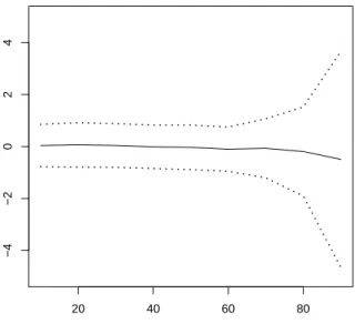
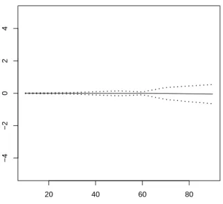
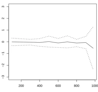
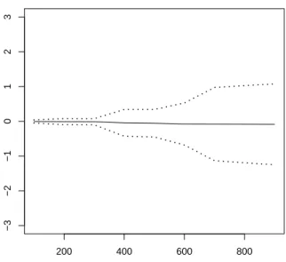
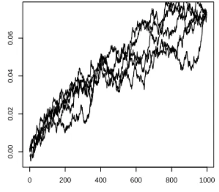
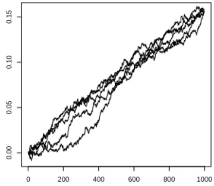
Our first set of results provides a very sharp approximation scheme; numerical evidence on exponential runs with lengthn= 1000 provide arelative error of the approximation of order less than 100% for the density of the first 800 terms when evaluated on the sample paths themselves, thus on the significant part of the support of the conditional density;
this very sharp approximation rate is surprising in such a large dimensional space, and it illustrates the fact that the conditioned measure occupies a very small part of the entire space. Therefore the approximation of the density ofXk1 is not performed on the sequence of entire spacesRk but merely on a sequence of subsets ofRk which bear the trajectories of the conditioned random walk with probability going to 1 as n tends to infinity; the approximation is performed ontypical paths.
The extension of our results from typical paths to the whole space Rk holds: conver- gence of the relative error on large sets imply that the total variation distance between the conditioned measure and its approximation goes to 0 on the entire space. So our results provide an extension of [33] and [29] who considered the case when k is of small order with respect ton; the conditions which are assumed in the present paper are weaker than those assumed in the just cited works; however, in contrast with their results, we do not provide explicit rates for the convergence to 0 of the total variation distance onRk.
It would have been of interest to consider sharper convergence criteria than the total variation distance; the χ2-distance, which is the mean square relative error, cannot be bounded through our approach on the entire spaceRk, since it is only handled on large sets of trajectories (whose probability goes to 1 an n increases); this is not sufficient to bound its expected value under the conditional sampling.
This paper is organized as follows. Section 2 presents the approximation scheme for the conditional density ofXk1 under the point conditioning sequence (S1,n =nan).In section 3, it is extended to the case when the conditioning family of events writes (U1,n =u1,n).
1.2. Random walks conditioned on their sum 19 The value of k for which this approximation is fair is discussed; an algorithm for the implementation of this rule is proposed. Algorithms for the simulation of random variables under the approximating scheme are also presented. Section 4 extends the results of Section 3 when conditioning on large sets.
The main steps of the proofs are in the core of the paper; some of the technicalities is left to the Appendix.
1.2 Random walks conditioned on their sum
1.2.1 Notation and hypothesis
In this section the point conditioning event writes En:= (S1,n=nan).
We assume thatXsatisfies the Cramer condition, i.e. Xhas a finite moment generating function Φ(t) :=EexptX in a non void neighborhood of 0. Denote
m(t) := d
dtlog Φ(t) s2(t) := d
dtm(t) µ3(t) := d
dts2(t)
The values ofm(t),s2 and µ3(t) are the expectation, the variance and the kurtosis of the tilted density
πα(x) := exptx
Φ(t) p(x) (1.1)
wheretis the only solution of the equationm(t) =αwhenα belongs to the support ofX.
Conditions on Φ(t) which ensure existence and uniqueness oftare referred to assteepness properties; we refer to [6] , p.153 and followings for all properties of moment generating functions used in this paper. Denote Πα the probability measure with densityπα. Remark 1. In many cases the functionφU(t) is not available in closed form, and conse- quently the same holds for the functionsm, s2andµ3. However tail probabilities are needed in safety surveys or in reliability studies; henceforth the real need is not on tail probabil- ities under the true (usually unknown ) model, but merely on some proxy of it, under which the tail probability estimate should have some conservative property. In a number of cases this may lead to a known model with rather simple forms for these functions. In other cases expansions of the functionφU(t) are available, leading to some approximation for the resulting derivatives. Inversion of m is feasible; inversion must be realized in a small interval around an. Hence the values ofs2(t) and µ3(t) for m(t) close to an can be calculated with good accuracy.
We also assume that the characteristic function ofX is in Lr for some r≥1 which is necessary for the Edgeworth expansions to be performed.
The probability measure of the random vector Xn1 on Rn conditioned uponEn is de- notedPnan.We also denote Pnan the corresponding distribution ofXk1 conditioned upon En; the vector Xk1 then has a density with respect to the Lebesgue measure on Rk for
1≤k < n,which will be denotedpnan. For a generic r.v. Zwith densityp,p(Z=z) de- notes the value ofpat point z.Hence, pnanxk1=pXk1 =xk1|S1,n =nan. The normal density function onRwith meanµand varianceτ atxis denotedn(µ, τ, x).Whenµ= 0 andτ = 1, the standard notationn(x) is used.
1.2.2 A first approximation result
We first put forwards a simple result which provides an approximation of the density pnan of the measure Pnan on Rk when ksatisfies (K1) and (K2) . Fori≤j denote
si,j :=xi+...+xj. Denotea:=an omitting the index nfor clearness.
We make use of the following property which states the invariance of conditional den- sities under the tilting: For 1 ≤ i ≤ j ≤ n, for all a in the range of X, for all u and s
p(Si,j =u|S1,n =s) =πa(Si,j=u|S1,n =s) (1.2) whereSi,j :=Xi+...+Xj together with S1,0=s1,0 = 0. By Bayes formula it holds
pna
xk1 =
k−1
Y
i=0
p(Xi+1=xi+1|Si+1,n =na−s1,i) (1.3)
=
k−1
Y
i=0
πa(Xi+1 =xi+1)πa(Si+2,n =na−s1,i+1) πa(Si+1,n=na−s1,i)
=
"k−1 Y
i=0
πa(Xi+1 =xi+1)
#πa(Sk+1,n =na−s1,k)
πa(S1,n =na) . (1.4) Denote Sk+1,n and S1,n the normalized versions of Sk+1,n and S1,n under the sampling distribution Πa.By (1.4)
pna
xk1=
"k−1 Y
i=0
πa(Xi+1 =xi+1)
# √
√ n n−k
πaSk+1,n = ka−s1,k
sa
√n−k
πaS1,n = 0 .
A first order Edgeworth expansion is performed in both terms of the ratio in the above display; see Remark6hereunder. This yields, assuming (K1) and (K2)
Proposition 2. For all xk1 in Rk
pna
xk1 =
"k−1 Y
i=0
πa(Xi+1=xi+1)
#
n ka−s1,k
s(ta)√ n−k
n(0)
r n
n−k (1.5)
1 + µ3(ta) 6s3(ta)√
n−kH3
ka−s1,k
s(ta)√ n−k
!!
+O 1
√n #
where H3(x) :=x3−3x.The value of ta is defined through m(ta) =a .
Despite its appealing aspect, (1.5) is of poor value for applications, since it does not yield an explicit way to simulate samples under a proxy of pna for large values ofk. The other way is to construct the approximation ofpna step by step, approximating the terms
1.2. Random walks conditioned on their sum 21 in (1.3) one by one and using the invariance under the tilting at each step, which introduces a product of different tilted densities in (1.4). This method produces a valid approximation of pna on subsets of Rk which bear the trajectories of the condition random walk with larger and larger probability, going to 1 as ntends to infinity.
This introduces the main focus of this paper.
1.2.3 A recursive approximation scheme We introduce a positive sequencenwhich satisfies
n→∞lim n
√
n−k=∞ (E1)
n→∞lim n(logn)2 = 0. (E2)
It will be shown thatn(logn)2 is the rate of accuracy of the approximating scheme.
We denote a the generic term of the convergent sequence (an)n≥1. For clearness the dependence in n of all quantities involved in the coming development is omitted in the notation.
Approximation of the density of the runs Define a density gna(y1k) on Rk as follows. Set
g0(y1|y0) :=πa(y1)
withy0 arbitrary, and for 1≤i≤k−1 define g(yi+1|yi1) recursively.
Setti the unique solution of the equation mi:=m(ti) = n
n−i
a−s1,i n
(1.6) wheres1,i:=y1+...+yi.The tilted adaptive family of densitiesπmi is the basic ingredient of the derivation of approximating scheme.Let
s2i := d2
dt2 (logEπmiexptX) (0) and
µij := dj
dtj (logEπmiexptX) (0), j = 3,4 which are the second, third and fourth cumulants ofπmi.Let
g(yi+1|y1i) =CipX(yi+1)n(αβ+a, β, yi+1) (1.7) be a density where
α=ti+ µi3
2s4i (n−i−1) (1.8)
β=s2i (n−i−1) (1.9)
andCi is a normalizing constant.
Define
gna(y1k) :=g0(y1|y0).
k−1
Y
i=1
g(yi+1|y1i). (1.10) We then have
Theorem 3. Assume (K1) and (K2) together with (E1) and (E2). Let Y1n be a sample with densitypna.Then
pnaY1k:=p(Xk1 =Y1kS1,n =na) =gna(Y1k)(1 +oPna(n(logn)2)). (1.11) Proof. The proof uses Bayes formula to write p(Xk1 =Y1kS1,n = na) as a product of k conditional densities of individual terms of the trajectory evaluated atY1k. Each term of this product is approximated through an Edgeworth expansion which together with the properties of Y1k under Pna concludes the proof. This proof is rather long and we have differed its technical steps to the Appendix.
DenoteS1,0 = 0 andS1,i:=S1,i−1+Yi.It holds
p(Xk1 =Y1kS1,n=na) =p(X1=Y1|S1,n =na) (1.12)
k−1
Y
i=1
p(Xi+1 =Yi+1|Xi1 =Y1i,S1,n=na)
=
k−1
Y
i=0
p(Xi+1=Yi+1|Si+1,n=na−S1,i) by independence of the r.v’s X0is.
Define ti through
m(ti) = n n−i
a−S1,i
n
a function of the past r.v’sY1i and set mi :=m(ti) and s2i :=s2(ti).By (1.2) p(Xi+1=Yi+1|Si+1,n=na−S1,i)
=πmi(Xi+1=Yi+1|Si+1,n=na−S1,i)
=πmi(Xi+1 =Yi+1)πmi(Si+2,n =na−S1,i+1) πmi(Si+1,n =na−S1,i)
where we used the independence of theXj’s under πmi.A precise evaluation of the dom- inating terms in this latest expression is needed in order to handle the product (1.12).
Under the sequence of densities πmi the i.i.d. r.v’s Xi+1, ...,Xn define a triangular array which satisfies a local central limit theorem, and an Edgeworth expansion. Under πmi,Xi+1 has expectationmi and variance s2i.Center and normalize both the numerator and denominator in the fraction which appears in the last display. Denoteπn−i−1the den- sity of the normalized sum (Si+2,n−(n−i−1)mi)/si√
n−i−1when the summands are i.i.d. with common density πmi. Accordingly πn−i is the density of the normalized sum (Si+1,n−(n−i)mi)/si√
n−i under i.i.d. πmi sampling. Hence, evaluating both πn−i−1 and its normal approximation at pointYi+1,
p(Xi+1 =Yi+1|Si+1,n =na−S1,i) (1.13)
=
√n−i
√n−i−1πmi(Xi+1 =Yi+1)
πn−i−1
(mi−Yi+1)/si
√n−i−1 πn−i(0)
:=
√n−i
√n−i−1πmi(Xi+1 =Yi+1)Ni Di.
The sequence of densities πn−i−1 converges pointwise to the standard normal density under (E1) which implies thatn−itends to infinity for all 1≤i≤k, and an Edgeworth
1.2. Random walks conditioned on their sum 23 expansion to the order 5 is performed for the numerator and the denominator. The main arguments used in order to obtain the order of magnitude of the involved quantities are (i) a maximal inequality which controls the magnitude ofmi for allibetween 0 andk−1 (Lemma 24), (ii) the order of the maximum of the Yi0s (Lemma 25). As proved in the Appendix,
Ni =n−Yi+1/si
√
n−i−1.A.B+OPna
1 (n−i−1)3/2
!
(1.14) where
A:= 1 + aYi+1
s2i(n−i−1)− a2
2s2i(n−i−1)+oPna(nlogn) n−i−1
!
(1.15) and
B:=
1− µi3
2s4i(n−i−1)(a−Yi+1)
− µi3−s4i
8s4i(n−i−1)− 15(µi3)2
72s6i(n−i−1) +OPna((logn)2)
(n−i−1)2
(1.16)
The OPna
1 (n−i−1)3/2
term in (1.14) is uniform upon (mi−Yi+1)/si√
n−i−1. Turn back to (1.13) and perform the same Edgeworth expansion in the denominator, which writes
Di =n(0) 1− µi3−s4i
8s4i(n−i) − 15(µi3)2 72s6i(n−i)
!
+OPna
1 (n−i)3/2
!
. (1.17) The terms in g(Yi+1|Y1i) follow from an expansion in the ratio of the two expressions (1.14) and (1.17) above. The gaussian contribution is explicit in (1.14) while the term exp µi3
2s4i(n−i−1)Yi+1 is the dominant term in B. Turning to (1.13) and comparing with (1.11) it appears that the normalizing factor Ci in g(Yi+1|Y1i) compensates the term
√n−i Φ(ti)√
n−i−1exp
−aµi3 2s2i(n−i−1)
,where the term Φ(ti) comes from πmi(Xi+1=Yi+1). Fur- ther the product of the remaining terms in the above approximations in (1.14) and (1.17) turn to build the 1 +oPnan(logn)2approximation rate, as claimed.Details are differed to the Appendix. This yields
p(Xk1 =Y1kS1,n=na) =1 +oPna
n(logn)2g0(Y1|Y0)
k−1
Y
i=1
g(Yi+1|Y1i) which completes the proof of the Theorem.
That the variation distance betweenPnan andGnan tends to 0 asn→ ∞is stated in Section 3.
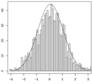
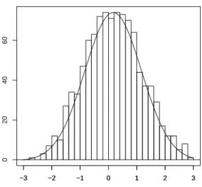
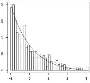
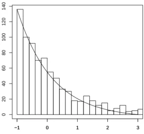
Remark 4. When theXi’s are i.i.d. with a standard normal density, then the result in the above approximation Theorem holds with k = n−1 stating that p(Xn−11 =xn−11 S1,n = na) = gnaxn−11 for all xn−11 in Rn−1. This extends to the case when they have an infinitely divisible distribution. However formula (1.11) holds true without the error term only in the gaussian case. Similar exact formulas can be obtained for infinitely divisible distributions using (1.12) making no use of tilting. Such formula is used to produce Figures 1.1, 1.2, 1.3 and 1.4 in order to assess the validity of the selection rule for k in the exponential case.
Remark 5. The density in (1.7) is a slight modification of πmi. The modification from πmi(yi+1)tog yi+1|y1iis a small shift in the location parameter depending both on aand on the skewness of p, and a change in the variance : large values of Xi+1 have smaller weight for large i, so that the distribution of Xi+1 tends to concentrate around mi as i approaches k.
Remark 6. In Theorem3 , as in Proposition2, as in Theorem9 or as in Lemma 25, we use an Edgeworth expansion for the density of the normalized sum of the n−ith row of some triangular array of row-wise independent r.v’s with common density. Consi