HAL Id: hal-00769274
https://hal.archives-ouvertes.fr/hal-00769274v1
Preprint submitted on 30 Dec 2012 (v1), last revised 27 Nov 2014 (v3)
HAL is a multi-disciplinary open access archive for the deposit and dissemination of sci- entific research documents, whether they are pub- lished or not. The documents may come from teaching and research institutions in France or abroad, or from public or private research centers.
L’archive ouverte pluridisciplinaire HAL, est destinée au dépôt et à la diffusion de documents scientifiques de niveau recherche, publiés ou non, émanant des établissements d’enseignement et de recherche français ou étrangers, des laboratoires publics ou privés.
Attack transients of an artificially blown clarinet : evolution of the sound amplitude for different blowing
pressure profiles
Baptiste Bergeot, André Almeida, Christophe Vergez, Bruno Gazengel, Ferrand Didier
To cite this version:
Baptiste Bergeot, André Almeida, Christophe Vergez, Bruno Gazengel, Ferrand Didier. Attack tran- sients of an artificially blown clarinet : evolution of the sound amplitude for different blowing pressure profiles. 2012. �hal-00769274v1�
Attack transients of an artificially blown clarinet : evolution of the sound amplitude for different blowing
pressure profiles
B. Bergeota,∗, A. Almeidaa, C. Vergezb, B. Gazengela, D. Ferrandc
aLaboratoire d’Acoustique de l’Université du Maine (LAUM-CNRS UMR 6613), Avenue Olivier Messiaen, 72085 Le Mans Cedex 9, France
bLaboratoire de Mécanique et Acoustique (LMA-CNRS UPR 7051), 31 Chemin Joseph Aiguier, 13402 Marseille Cedex 20, France
cLaboratoire d’Astrophysique de Marseille (LAM-CNRS-INSU UMR 7326), Pôle de l’Étoile Site de Château-Gombert / 38, rue Frédéric Joliot-Curie 13388 Marseille Cedex 13, France
Abstract
The work presented is an experimental study on the influence of the blowing pressure profile on the attack transient of the clarinet. A clarinet mouthpiece connected to a straight cylindrical pipe was played by an artificial mouth in which the blowing pressure can be accurately controlled through time.
Piece-wise linear time profiles are used for the blowing pressure. The observed oscillation thresh- old as well as the envelope of the mouthpiece pressure are analyzed for different configurations and compared to predictions from the Raman model. Differences between predictions and observations are interpreted in terms of bifurcation delay.
Firstly, the pressure is increased constantly at several different rates until the oscillations are well established in the resonator. The oscillations are seen to start at a value of the blowing pressure which is higher than expected from a stationary analysis. This value is as high as the slope of the pressure increase is higher.
In a second time, a fast linear increase of the blowing is suddenly stopped at a target pressure value. In this case, the oscillations are seen to start close to the stop in pressure increase, or before this instant. The transient time of the resonator pressure is constant.
∗Corresponding author,baptiste.bergeot@univ-lemans.fr
Keywords: Musical acoustics, Clarinet-like instruments, Transient processes, Iterated maps, Dynamic Bifurcation, Bifurcation delay.
1 Introduction
This work is an experimental study of the attack transients in a clarinet-like instrument (mouthpiece and barrel of a real clarinet connected to a simple cylinder, see Fig. 1(a)) blown using a pressure controlled artificial mouth (PCAM). A detailed description of the PCAM is made in section 3. The general aim is to observe the time evolution of the envelope of the acoustic pressure inside the mouth- piece during the attack transient (including the oscillation threshold) for simple time profiles of the blowing pressure. More precisely, we focus on links between the characteristics of the attack transient of the pressure inside the mouthpiece and characteristics of the time evolution of the blowing pressure.
Two different profiles are used for the blowing pressure. The first is a slowly increasing, then decreasing pressure leading to an academic study of the influence of the increase rate (the slope) of the blowing pressure on the attack transient of the acoustic pressure inside the mouthpiece. The presentation of the experiment and the ensuing results are presented in section4. In general, oscillations inside the resonator are first observed at a much higher blowing pressure than the static oscillation threshold predicted in the context of Raman model [1,2,3,4,5] (see section2 for a brief description of the this model). The difference between the two values increases with the slope of the blowing pressure. This observation may be related to the phenomenon of bifurcation delay [6, 7]. Finally, we show a comparison between experimental results and results obtained from numerical simulations of Raman model, presented in section2.
In section5, a slightly more realistic mouth pressure profile is chosen. Its time evolution is divided into two parts. In a first phase the blowing pressure increases at a higher rate than ones used in section 4. The second phase is characterized by a constant blowing pressure. Consequences on the attack transient of the sound are discussed.
2 Elements of theory of clarinet behavior
Raman model simplifies the structure of an auto-oscillating instrument to a maximum extent so that a square-wave propagates in the resonator and reflects passively at the open end and through a nonlinear function at the mouthpiece end. This allows to estimate static oscillation thresholds and amplitudes of the permanent regime as a function of the playing parameters (blowing pressure Pm and lip force ζ).
The seminal article from Mc Intyre et al. [8] proposes a general model for self-sustainded musical
instruments such as the clarinet. This model divides the instrument into two elements: the exciter and the resonator. The exciter of a clarinet is the reed-mouthpiece system characterized by the so- called nonlinear characteristics of the exciter, a function relating the flow U across the reed entrance to the pressure difference ∆P = Pm−P using Bernoulli equation [2]. The resonator is the bore of the instrument described by its reflection function r(t). The solutions P(t) and U(t) depend on the control parameters: Pm representing the mouth pressure andζ which is related to the opening of the embouchure. In this work we use a fixed embouchure, the control parameter ζ is therefore constant.
2.1 Nonlinear characteristics of the exciter
Assuming that the reed behaves as an ideal spring without damping or inertia, changes in pressure induce an instant movement of the reed and an instant change in the flowU(t). This can therefore be related to the pressure differencePm−P(t) through the nonlinear characteristics of the exciter:
U =
ζ
Zc (PM −∆P) s
|∆P|
PM sgn(∆P), (1a)
if ∆P < PM ;
0, if ∆P > PM, (1b)
where PM is the static closing pressure of the reed. The control parameter ζ is a non dimensional parameter, its expression is :
ζ =Zc S r 2
ρPM, (2)
where S is the cross-section of the reed channel at rest, ρ the density of the air and Zc =ρc/Scyl the characteristic impedance of the cylindrical resonator of cross-section Scyl.
It can be noticed [5] that the coordinates of the maximum flow of the nonlinear characteristics are linked to the reed parameters through:
Pmax= PM
3 , (3)
and
Umax= 2 3√
3 PM
Zc ζ. (4)
2.2 The resonator
In Raman model the resonator is a perfectly cylinder in which the dispersion is ignored and the losses are assumed to be frequency independent [1, 2, 3, 4, 9, 5]. With these assumptions, the reflection function seen from the mouthpiece becomes a simple delay with sign inversion (multiplied by an attenuation coefficient λ). Using the variables P+ = 12(P+ZcU) and P− = 12(P −ZcU) (outgoing and incoming waves respectively) instead of the variablesP andU, the system can be simply described by the following equation:
P+(t) =G λP+(t−τ)
, (5)
where τ = 2l/c is the round trip time of the pressure perturbation with velocityc along the resonator of length l. The function G is obtained by substituting the variables P and U by variables P+ and P− in equation (1) . An explicit expression can be found in Taillardet al. [10].
The attenuation coefficientλtakes into account the visco-thermal losses along the resonator, which at low frequencies are dominant over the radiation losses. It can be approximated by the expression:
λ=e−2αl, (6)
where α is the damping factor [11]:
α≈3·10−5p
f /R. (7)
R is the radius of the bore: R = 7.5·10−3 m in our experiment and f is the frequency in Hz. In the context of Raman model the damping factor αis constant, calculated at the playing frequency.
2.3 Static oscillation threshold
A study of the stability of the fixed points of the functionG, based on the usual static bifurcation theory (i.e. assuming that the mouth pressure is constant along the time), gives an analytical expressionPmt of the static oscillation threshold [12]:
Pmt= 1 9
tanh(αl)
ζ +
s 3 +
tanh(αl) ζ
2
2
PM. (8)
We add the word static to the usual name oscillation threshold to emphasize that the analytical expression is obtained from the static bifurcation theory which assumes a constant blowing pressure.
In practice this can correspond to increasing the pressure to a constant value and waiting for the oscillating regime to be fully developed [13].
3 Experimental setup : the pressure controlled artificial mouth (PCAM)
The experimental setup is made of a controlled artificial mouth [14,15]. The artificial mouth consists of a Plexiglas box. The mouthpiece and the barrel are rigidly attached to the box. Resonators (for example, a real clarinet or a simple cylinder as in our experimenta) can be attached to the other end of the barrel (see Figure. 1(a)).
Figure 1: (color online) (a) General view of the artificial mouth. (b) Lateral view of the mouthpiece placed in the artificial mouth. The lip is shown in the position used for the measurements in this article.
The machinery of the controlled artificial mouth is based on a high-precision regulation of the air pressure in the Plexiglas box. This regulation enables to control the blowing pressure around a target:
a fixed value or around a value whose evolution in time is slow (like slowly varying ramps as in this present work). The experimental setup is presented in Figure 2.
aWe use a plastic cylinder,l= 0.52m long including the barrel of the clarinet.
Computer + dSpace hardware
servo valve Compressed air
(~ 6 bars)
Pressure reducer
P1
Qi, P2 i
Pressure sensor Artificial
mouth + Instrument
Pm
Air tank Flow meter
Figure 2: (color online) Principle of the pressure controlled artificial mouth. Through a control algo- rithm implemented on a DSP card, the volume flow through the servo-valve is modified every 40µs in order to minimize the difference between the measured and the target mouth pressure.
A servo-valve is connected to a compressed air source through a pressure reducing valve. The maximum pressure available is around 6 bars, and the pressure reducer is used to adjust the pressure P1 upstream the servo-valve. The servo-valve is connected to the entrance of the artificial mouth itself, a chamber with internal volume of 30 cm3 where the air pressure Pm is to be controlled. The artificial mouth blows into the clarinet. An air tank (120L) is inserted between the servo-valve and the artificial mouth in order to stabilize the feedback loop during slowly varying onsets. The air tank is replaced by a much smaller volume (∼2L) when faster varying targets are tested.
The principle of the control is as follows: through a control algorithm implemented on a DSP card, the volume flow through the servo-valve is modified every 40 µs in order to minimize the difference between the measured and the target mouth pressure.
The force applied by the lip on the reed also has an influence on the value of the oscillation threshold.
This force is maintained constant during the experiment using an artificial locked to a constant position (cf. Figure 1(b)).
Finally, a flowmeter is placed at the entrance of the artificial mouth in order to measure the nonlinear pressure/flow characteristic defined in equation (1).
Table 1: Estimation of the slope for each occurrence of each experiment. Averages calculated from the three values obtained for each experiment are also listed.
Experiment 1 2 3 4 5 6
Values of k (kPa/s) (incr. blowing pressure)
1st time 0.100 0.140 0.233 0.751 1.557 2.681 2nd time 0.100 0.140 0.233 0.752 1.557 2.712 3rd time 0.100 0.140 0.233 0.753 1.559 2.711 Average 0.100 0.140 0.233 0.752 1.558 2.702
4 Slowly time-varying blowing pressure
4.1 Description of the experiments
The procedure of the experiment is as follows: starting from a small value (0.2 kPa in our experiment) the mouth pressure Pm(t) is increased at a constant rate k (the slope) up to a value beyond the oscillation threshold. The mouth pressure is then decreased with a symmetric slope(k′=−k). During the experiment, the mouth pressurePm(t), the pressure in the mouthpiece P(t)and the incoming flow U(t) are recorded, and the RMS value PRM S(t) of the pressure in the mouthpiece is then calculated.
Fig.3 shows an example of the time profile of Pm,P and PRM S withk= 0.1 kPa/s.
Figure 3: Time evolution of the mouth pressure Pm , the pressure inside the mouthpiece P and its RMS valuePRM S. The slope kof the mouth pressure is equal to 0.1 kPa/s.
The experiment is repeated for different values of the slopekand three times for each value. Values of the slope are estimated using a linear fit and shown in Tab.1. We can see that the use of the PCAM provides a very good repeatability on the increase/decrease rate of the blowing pressure.
The aims of this section are:
• To compare the values Pm at which the oscillating resonator rises up from the background
noise (hereafter referred to Pstart) to the analytical static oscillation threshold Pmt defined through equation (8) and calculated using parameters obtained from the experimental nonlinear characteristics;
• To determine whetherPstart depends on the slope kof the blowing pressure;
• To study the duration of the attack transient of P with respect to time and to the blowing pressure (focusing on the study with respect to the blowing pressure);
• To study how this duration changes when the slopek increases.
Different objective indicators are estimated in order to acheive these aims. These indicators are presented in Fig.4.
Three time indicators are first estimated: tstart,tend and τ. tstartand tend correspond respectively to the beginning and the end of the attack transient of the acoustic pressureP(t)inside the mouthpiece.
tstart is the time whereP(t) rises up from the background noise, it is defined as the time at which the RMS envelope PRM S(t) reaches a threshold equal to four times the average of the noise background.
tend is estimated as the time where there is a local minimum of the second derivative of the RMS envelope [17]. tstart andtend define the duration of the attack transient (∆t)PRM S of the sound inside the mouthpiece calculated on the RMS envelope PRM S:
(∆t)PRM S =tend−tstart. (9)
Assuming that the growth of the oscillations (here the growth of the RMS envelope of the acoustic pressure inside the mouthpiece) is exponential, we estimate its time constantτ.
Then, indicators describing the evolution of the RMS envelopePRM S as a function of the blowing pressurePm are determined. Pstart andPend are the values of the blowing pressure at timeststart and tend.
The value Pstart can be questioned due to its intrinsic arbitrary nature. In fact there is no way to determine exactly the instant at which the oscillations start. Should the oscillations start in a completely noise-free environment, it would be straight-forward to determine an amplitude of the oscillations at the playing frequency of the instrument. In our case, however, some energy exists at this frequency due to the turbulence of the flow before any oscillation is present. It is thus difficult to determine whether the oscillations are excited by the stochastic component of the pressure or by an intrinsic instability of the system driven by a variable parameter [7].
Otherwise, the choice of the constant factor applied to the noise (4 in our case) can be seen as arbitrary. However keeping this value the same for all experiments should provide values ofPstart that
can be compared for different trials. In fact the noise level is quite reproducible, and thus the reference value corresponding toPstart follows a similar trend.
Pstart andPend define the duration of the attack transient of the sound inside the mouthpiece with respect to blowing pressurePm:
(∆P)PRM S =Pend−Pstart. (10)
Given that the blowing pressure is an affine function of time,PRM S can be described using similar functions either of time or blowing pressure. The exponential coefficient of PRM S as a function of the blowing pressure (τPm) is then proportional to the time constant.
Attack transient
• t
• Pstart
tstart Pend
tend
∼eτt Pm PRM S
Attack transient
Pm
PRM S
•
•
Pstart Pend
∼e
Pm τPm
Figure 4: Outline schematic showing the definition of the different indicators. At the top: schematic representation of the the blowing pressure Pm and of the RMS envelope PRM S of the pressure inside the mouthpiece as functions of time. Illustrations of tstart, tend, Pstart, Pend and τ. At the bottom:
schematic representation of PRM S as a function of the Pm. Definition ofτPm.
4.2 Estimation of the static oscillation threshold
An estimation of the theoretical static oscillation thresholds of the clarinet system can be calculated using equation (8) by introducing the correct parameters α, ζ and PM in equation 1. The damping
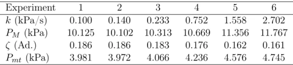
Table 2: Averages of the slopek, of the parameters PM, ζ and of the static oscillation threshold Pmt
obtained for increasing and decreasing blowing pressure.
Experiment 1 2 3 4 5 6
k(kPa/s) 0.100 0.140 0.233 0.752 1.558 2.702 PM (kPa) 10.125 10.102 10.313 10.669 11.356 11.767 ζ (Ad.) 0.186 0.186 0.183 0.176 0.162 0.161 Pmt (kPa) 3.981 3.972 4.066 4.236 4.576 4.745
factor α is calculated, through equation (7), at the playing frequency. The parameters PM and ζ are determined from the coordinates of the maximum of the characteristic curve (Pmax, Umax) through equations (3) and (4).
Fig. 5shows an example of an experimental nonlinear characteristic (gray line). As stated previ- ously in [18,19,13], due to the viscoelastic behavior of the reed, the two characteristics, for increasing and decreasing blowing pressure, are different.
The focus of this article is the growth of the oscillations for increasing blowing pressures. Therefore, the reed parameters needed for the calculation of the static oscillation threshold are those estimated from the characteristics obtained for increasing pressures. The averages ofPM, ζ and Pmt calculated from the three values obtained for each experiment are summarized in Tab. 2.
Due to the response time of the flowmeter (≈ 0.3s), the experimental nonlinear characteristics corresponding to experiments 4, 5 and 6 cannot provide an optimal estimation of the parameters.
The closing pressure PM and of the static oscillation threshold Pmt are overestimated. Therefore, the parameters PM, ζ and Pmt used in the rest of this paper are averages obtained with the slower increasing blowing pressures (experiment 1, 2 and 3). Their numerical values are: PM = 10.18 kPa, ζ = 0.185 and using equation (8) Pmt = 4.01kPa. For decreasing blowing pressures the average static oscillation threshold is 3.95 kPa. The viscoelastic behavior of the reed has therefore a small effect on the value of the static oscillation threshold.
In Fig. 5 the comparison between the experimental nonlinear characteristics (gray line) and the analytical one (black line) calculated using equation (1) shows a good agreement. Therefore the estimation of the parametersζ and PM appears to be satisfactory.
-1 0 1 2 3Mx 44 6 7 0
5 10 15 M20y
Pm−P (kPa)
U(L/min)
Experimental Theoretical
Figure 5: Graphical representation of the experimental nonlinear characteristics of the exciter (gray line) for increasing and decreasing blowing pressure and comparison with model (black line) for in- creasing blowing pressure. In this example the increase rate k of the blowing pressure is equal to 0.1kPa/s.
4.3 Experimental results
In Fig. 6, the RMS envelope PRM S is plotted as a function of the mouth pressure Pm for different slopes of the blowing pressure. First of all, it is worth noting that for all values of the slopek, the state reached at the end of the transient belongs to the same periodic branch (slight repeatability errors aside). Fig.6highlights an hysteretic cycle: periodic sound emerges from the background noise during the increasing phase at a higher value of Pm than the value at which it stops during the decreasing phase. In the light of the results presented in Tab. 2, this difference cannot be explained only by the change of the reed parameters during the ascending and descending phase of the blowing pressure. In section4.4the comparison between experiment and numerical simulations will confirm this hypothesis.
Finally, Fig.6also shows that a direct Hopf bifurcation takes place, since the RMS envelope approaches zero continuously as the blowing pressure decreases.
3 3.5 Pmt 4.5 5 5.5 6 6.5 7 0
0.5 1 1.5 2 2.5 3 3.5
Pm (kPa) PRMS(kPa)
k6
k5
k4
k3
k2
k1
Figure 6: Graphical representation of PRM S as a function of Pm for different values of the slope k:
k1 < k2 < ... < k6. Arrows represent the direction of the mouth pressure time evolution and highlight an hysteretic cycle.
The main results presented in this section are summarized in the example depicted in Fig.7.
3.5 Pmt 4.5 Pstart 5.5 6 6.5 10−2
100
k2
3.5 Pmt 4.5 Pstart 5.5 6 6.5
10−2 100
k3
3.5 Pmt 4.5 5 Pstart 5.5 6 6.5
10−2 100
k4
3.5 Pmt 4.5 5 Pstart 6 6.5
10−2 100
k5
3.5 Pmt 4.5 5 Pstart 6 6.5
10−2 100
Blowing pressurePm(kPa) k6
3.5 Pmt 4.5 Pstart 5.5 6 6.5
10−2 100
k1
PRM S[Pm](kPa)
∼ePm/τPm
PRM S[Pm=Pstart] PRM S[Pm=Pend] Bifurcation delay
Figure 7: Graphical representation ofPRM S,Pstart,Pend andePM/τPm. One example is shown for each value of the slope k. As previously k1 < k2 < ... < k6. A logarithmic scale is used for the ordinate axis.
The observations that can be drawn from these graphics can be resumed as follows:
• Periodic sound always starts at a higher value (Pstart) of the blowing pressure than static oscil- lation threshold Pmt. This observation is interpreted as a case of bifurcation delay[6,7]
• The difference betweenPmtandPstartincreases as the slopekof the blowing pressure is increased.
These results are studied more precisely in section4.3.1.
• The attack phase of the pressure P inside the mouthpiece, when plotted against the blowing pressure, increases as an exponential growth.
• The attack phase takes place in a range of values of Pm which increases with the slope k of the blowing pressure. See 4.3.2 for a more rigorous study of these two previous points.
4.3.1 Beginning of the attack transient of the acoustic pressure inside the mouthpiece This section looks in more detail into the apparent delay between the start of the oscillations in the resonator pressure (Pstart) and the expected start (the static thresholdPmt).
The indicator ∆G=Pstart−Pmt is plotted with respect to the slope kin Fig. 8where all records are represented. We notice a good repeatability of the measurement. Indeed, there is little dispersion between the three tests of each slope k. As suggested by Fig. 6 and Fig. 7, the gap ∆G is always greater than zero and increases with the slopek.
0 0.5 1 1.5 2 2.5 3
3.5 Pmt
4.5 5 5.5 6
∆G:bifurcation delay
k (kPa/s) Pstart(kPa)
Figure 8: Graphical representation of Pstart (◦) as a function of the slope k. The shaded portion depicts the bifurcation delay ∆G.
The fact that the values of Pstart are always larger than static oscillation threshold Pmt can be explained by the intrinsic difference between the system described by the static theory where the blowing pressurePmis assumed to be constant (this is astaticcase) and the system used in experiments where the blowing pressure is increasing (this is adynamic case).
Recent theoretical and experimental works [6,20, 21] on dynamical nonlinear systems show that, in dynamic cases (as in our experiments), the oscillations start significantly after thestatic theoretical threshold has been reached. This phenomenon is known under the name ofbifurcation delay ordynamic bifurcation. In [7], the authors present a mixed analytical/numerical study of the lossless model of the clarinet (Raman model with λ = 1) taking into account a time-varying blowing pressure. We see
that, in a noisy system (numerical noise, i.e. round off errors of the computer), the bifurcation delay increases with the slope of the blowing pressure, as the variable∆G in our experiment.
Therefore, the variable∆G is interpreted afterwards as a measurement of the bifurcation delay in our system, although some caution might be need while using this value.
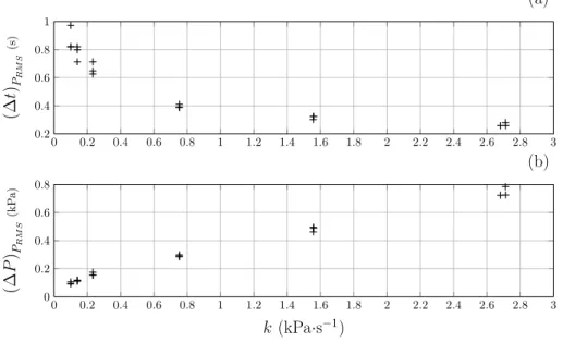
4.3.2 Duration of the attack phase of the acoustic pressure inside the mouthpiece We focus here on the duration of the attack transient of the pressure P inside the mouthpiece of the instrument measured both in time and blowing pressurePmt(t). For this,(∆t)PRM S and(∆P)PRM S are plotted in Fig. 9 as functions of the slopek. Fig. 9(a) shows the evolution of (∆t)PRM S, the duration of the attack transient deccreases with the slope k. On the contrary, Fig.9(b) shows that (∆P)PRM S appears to increase with the slopek. This means that even if the duration (with respect to time) of the attack transient of the acoustic pressure inside the mouthpiece decreases withk, the blowing pressure sees a wider variation during this attack transient.
This previous result is attested by the Fig. 10(a) where the parameter τ is plotted as a function of the slope k. Indeed, the time constant τ of the exponential growth of the RMS envelope decreases withk unlike the constantτPm which increases (cf. Fig. 10(b)).
0 0.2 0.4 0.6 0.8 1 1.2 1.4 1.6 1.8 2 2.2 2.4 2.6 2.8 3
0.2 0.4 0.6 0.8 1
(∆t)PRMS(s)
(a)
0 0.2 0.4 0.6 0.8 1 1.2 1.4 1.6 1.8 2 2.2 2.4 2.6 2.8 3
0 0.2 0.4 0.6 0.8
k (kPa·s−1) (∆P)PRMS(kPa)
(b)
Figure 9: Graphical representation of(∆t)PRM S (a) and (∆P)PRM S (b) with respect to the slopek.
0 0.2 0.4 0.6 0.8 1 1.2 1.4 1.6 1.8 2 2.2 2.4 2.6 2.8 3 0.05
0.1 0.15 0.2 0.25 0.3
τ(s)
(a)
0 0.2 0.4 0.6 0.8 1 1.2 1.4 1.6 1.8 2 2.2 2.4 2.6 2.8 3
0 0.04 0.08 0.12 0.16
k(kPa·s−1) τPm(Pa)
(b)
Figure 10: Graphical representation of the parameters τ (a) andτPm (b) with respect to the increase ratek of the blowing pressure.
4.4 Comparison with Raman model
In this section, previous experimental results are compared to numerical computations using Raman model (using equation 5). The simulation uses the experimental blowing pressure Pm(t) and the reed parameters ζ and PM estimated in section 4.2 to plot PRM S envelopes and compare them with experimental signals in Fig.11. As in experiments, hysteretic cycles and bifurcation delays are present in simulations.
The behavior of the model is qualitatively the same as that of the real system. The comparison between the indicators (Pstart,Pend,τPmandτ) previously estimated on real signals and those obtained on simulated signals (see Fig. 12,13and14) confirms the close proximity between the behavior of the model and that of the instrument.
However, a closer look reveals a few differences. Fig. 12 shows that the values Pstart and Pend estimated on numerical simulations are always smaller than the experimental ones. A possible reason for this is that the static oscillation threshold deduced from PM and ζ is underestimated. Indeed, in Fig. 11(b), the decreasing slope of simulations k1, k2 and k3 shows an extinction of the sound close to the static oscillation threshold Pmt = 4.01kPa. On the other hand, for experimental signals (cf.
Fig.11(a)), the extinction is close to 4.5 kPa which can indicate that the static threshold is close to this value. Underestimation is common when using a fit of the non-linear characteristics [22]. Nevertheless, the delay in the start of the oscillations still be occurs even if the static threshold is close to 4.5 kPa.
Moreover, its dependence on the variation of the parameter kis unchanged.
3 3.5 Pmt 4.5 5 5.5 6 6.5 7 0
1 2 3 4 5 6 7
Pm (kPa) PRMS(kPa)
(a) Experiment
k6
k5
k4
k3
k2
k1
3.5 Pmt 4.5 5 5.5 6 6.5 7
0 1 2 3 4 5 6 7
Pm (kPa) PRMS(kPa)
(b) Simulation (Raman model)
k6
k5
k4
k3
k2
k1
Figure 11: Graphical representation of PRM S as function of Pm for each values of the slope k. (a) Experimental signals, (b) signals generated by the numerical simulation of Raman model using the parameters ζ and PM estimated experimentally (cf. section 4.2) as well as the measured blowing pressure signal Pm(t).
0 0.5 1 1.5 2 2.5 3
3.5 Pmt
4.5 5 5.5 6 6.5 7 7.5
k (kPa·s−1)
Pend: experiment Pstart: experiment Pend: simulation Pstart: simulation
Figure 12: Graphical representation of Pstart (◦) andPend (+) as a function of the slope k. The black marks are related to values obtained experimentally and the gray marks are related to values obtained on numerical simulation of Raman model.
0 0.2 0.4 0.6 0.8 1 1.2 1.4 1.6 1.8 2 2.2 2.4 2.6 2.8 3 0.2
0.4 0.6 0.8 1
(∆t)PRMS(s)
(a)
Experiment Simulation
0 0.2 0.4 0.6 0.8 1 1.2 1.4 1.6 1.8 2 2.2 2.4 2.6 2.8 3
0 0.2 0.4 0.6 0.8
k (kPa·s−1) (∆P)PRMS(kPa)
(b)
Experiment Simulation
Figure 13: Graphical representation of (∆t)PRM S (a) and (∆P)PRM S (b) with respect to the slope k.
(◦) simulation and (+) experiment.
0 0.2 0.4 0.6 0.8 1 1.2 1.4 1.6 1.8 2 2.2 2.4 2.6 2.8 3
0 0 0.1 0.2 0.3
τ(s)
(a)
Experiment Simulation
0 0.2 0.4 0.6 0.8 1 1.2 1.4 1.6 1.8 2 2.2 2.4 2.6 2.8 3
0 0.04 0.08 0.12 0.16
k(kPa·s−1) τPm(Pa)
(b)
Experiment Simulation
Figure 14: Graphical representation of the parameters τ (a) andτPm (b) with respect to the increase ratek of the blowing pressure. (◦) simulation and (+) experiment.
These numerical simulations also provide a strong indication that the hysteresis in the envelope of the resonator pressure cannot be due uniquely to the viscoelastic change in reed properties. In fact the simulations are run with constant reed parameters (leading to a constant ζ) and a hysteresis is still observed.
5 Fast transient to a constant blowing pressure
The previous section highlighted the presence of a delayed start of oscillations in the context of a continuously variable blowing pressure. In the current section a slightly more realistic evolution of the blowing pressure is used in order to investigate the effect of a sudden stop in the pressure increase.
Such a time profile ofPm(t) can be seen as a simplistic model of an attack curve of a real musician.
5.1 Description of the experiment
In the following measurements, the time evolution of the blowing pressure is divided into two parts.
During the first part, the blowing pressure increases at a rate larger than the ones used in section 4.
In the second part, the blowing pressure is kept close to a constant value. An example is shown in Fig.15.
The procedure is as follows: the blowing pressurePm starts from a low level (≈0.1 kPa), increases during certain time (will be hereafter referred as(∆t)Pm), reaches a target value (≈7 kPa) and remains constant. The experiment is repeated for different values of (∆t)Pm (the commands given for it to the PCAM are: 0.05s, 0.2s, 0.5s and 1s corresponding respectively to experiments numbered 1, 2, 3 and 4, cf. Tab. 3) and fifteen times for each value of (∆t)Pm.
During the experiment the blowing pressure Pm and the pressure P inside the mouthpiece are recorded (see Fig. 15). The mean flow U entering the instrument is also recorded but, as in section 4 in fastest cases, the response time of the flowmeter is too slow to expect a good estimation of the model’s parameters. Moreover, the opening of the embouchure is different from that of section4. Thus the parameters estimated in section 4.2cannot be used in the current measurements.
0 0.1 0.2 0.3 0.4 0.5 0.6 0.7 0.8 0.9 1 1.1 1.2
−8
−6
−4
−2 0 2 4 6 8
Time (s)
Pressure(kPa)
Mouthpiece pressureP(t) Blowing pressurePm(t)
Figure 15: Graphical representation of the the measured signals: the blowing pressure Pm(t) (solid black line) and the pressure inside the mouthpiece P(t) (solid gray line).
The main aim of this section is to study the influence of the duration of the increase phase of the blowing pressure(∆t)Pm on the attack transient of the mouthpiece pressureP(t). The target value of the blowing pressure is the same in each experiment.
As in the previous section, a few indicators are extracted from the measured signals, although with a few differences. The growing phase of Pm is detected from a threshold on numerical derivative of Pm. Two reference points,(tbeg)Pm and(tend)Pm, result from this detection, and allow to estimate the duration of the transient of the blowing pressure:
(∆t)Pm = (tend)Pm−(tbeg)Pm. (11) Assuming that the growth ofPm is linear, its slopek is estimated between the times(tbeg)Pm and (tend)Pm.
The attack transient of the pressureP inside the mouthpiece is here described by the amplitude of the first harmonic PH1(t) instead of the RMS envelope PRM S(t) as it can detect the emergence of the sound at lower amplitudes. In fact, the noise background is lower if calculated at a narrow range of frequencies than for the RMS envelope which is wideband. Fig. 16shows a comparison between the two envelopes PRM S(t) and PH1(t) for different values of(∆t)Pm.
(∆t)Pms
(a)
0 0.1 0.2 0.3 0.4 0.5 0.6 0.7 0.8 0.9 1 1.1 1.2
−4
−2 0 2 4 6 8 10
Pmstransient Pms(kPa)
(∆t)PH1
T
(b)
0 0.1 0.2 0.3 0.4 0.5 0.6 0.7 0.8 0.9 1 1.1 1.2
10−5 10−4 10−3 10−2 10−1 100 101 102
Time (s)
Pmstransient PRMStransient PH1
refs pt. onPH1
Figure 16: Example of the time evolutionPH1(t)andPRM S(t)for each value of(∆t)Pm. A logarithmic scale is used for the ordinate axis.
A low (noise background close to the note end) and high value (absolute maximum) of the logarithm
envelope log [PH1/Pref] (Pref = 1kPa) are first detected. The first value of log [PH1/Pref] crossing the midpoint between these two previous values is used as a reference time t50. Four other points are detected onlog [PH1/Pref]: t10,t30,t70andt90. Using these reference points the duration of the attack transient of the pressureP is defined as:
(∆t)PH
1 =t90−t10. (12)
Next, the durationT defines the difference in time between the beginning of the attack transient ofP and the stop of the growth of the blowing pressure:
T =t10−(tend)Pm (13)
An illustration of these previous indicators is depicted in Fig. 17.
0 0.2 0.4 0.6 0.8 1 1.2 1.4 1.6 1.8
10−5 10−4 10−3 10−2 10−1 100 101
102 Command for(∆t)Pms :from 0.05s to 1s
Time (s)
PRMS
PH1
Figure 17: (a) Graphical representation of the static blowing pressurePm, the gray area represents the duration (∆t)Pm of the transient of Pm. (b) Plot of PH1(t) using a logarithmic scale for the ordinate axis, the hatched area depicts the duration (∆t)PH
1 of the attack transient of the pressure P inside the mouthpiece. The duration T, defined by equation (13), is also represented.
Finally, assuming that the attack phase consists of an exponential growth where PH1(t)∼et/τH1, the time constant τH1 is estimated as the slope oflog [PH1(t)/Pref]between t30 andt70.
5.2 Experimental results
The indicators defined above are calculated for each trial. Some of the original trials are removed from the analysis if the fundamental frequency f0(t) is higher than expected (≥200Hz, whereas the expected playing frequency is around 160Hz) for a long period of time during the attack phase. This
corresponds to squeaks or higher regimes which afterwards decay to the fundamental. The trials where the attack phase lasts longer than 400ms are also removed.
First of all, Tab.3shows a good agreement between the command and the measurement of(∆t)Pm. This indicates that the control of the PCAM works even for rapid variations of the blowing pressure.
However, for the fastest one (experiment 1) the difference between the command and measurement is about 50% of the command. Tab. 3 also shows a good repeatability of the measurement of the slope k of the blowing pressure during the increasing phase.
In the remaining of this paper, the figures (except Fig.20) will show the averages of the indicators (written with an overline) plus or minus the standard deviations with respect to the average of the measured (∆t)Pm noted(∆t)Pm.
Table 3: Averages and standard deviations of the measured(∆t)Pm andkobtained for each command given to the PCAM for (∆t)Pm.
Experiment 1 2 3 4
Command for (∆t)P
m (s) 0.05 0.2 0.5 1
Average of measured(∆t)Pm: (∆t)Pm (s) 0.0747 0.2047 0.4590 0.9168 Standard deviation of measured (∆t)P
m (s) 0.0100 0.0108 0.0029 0.0060 Average of measuredk: k (kPa/s) 80.7354 29.9284 13.4157 7.4133 Standard deviation of measured k (kPa/s) 7.6354 1.0262 0.2061 0.0378
The example depicted in Fig.16 shows that the amplitude of the sound grows exponentially at the beginning of the attack. Moreover, we can see that the time constant τH1 looks constant regardless to the value of (∆t)Pm.
Fig.18(a) shows the average plus or minus the standard deviation of the time constantsτH1obtained for each value of (∆t)Pm. Fig. 18 confirms the observations made in Fig. 16: the time constant τH1 does not depend on the value of(∆t)Pm. Moreover, we can see that the duration(∆t)PH
1 of the attack transient plotted in Fig.18(b) also does not depend on(∆t)Pm. The repeatability of the measurement is good for bothτH1 and (∆t)PH
1: the standard deviation is between 7% and 14% of average.
In this particular case of a fast linear growth of the blowing pressure followed by a stationary phase, these results highlight that there is no "soft or fast" attack. The duration of the attack transient of sound is roughly the same whatever the duration of the transient of the blowing pressure. The only impact of increasing (∆t)Pm is a rightward shift of the curve of PH1 (cf. Fig. 16).
0.075 0.205 0.460 0.917 3
4 5 6·10−2
τH1(s)
(a)
0.075 0.205 0.460 0.917
0.15 0.2 0.25 0.3 0.35 0.4
(∆t)Pm (s) (∆t)PH1(s)
(b)
Figure 18: Average plus or minus the standard deviation of (a) the time constant τH1 and (b) the duration of the attack transient (∆t)PH
1 obtained for each value of (∆t)PH
1.
This result differs from results presented in section 4.3.2 (Fig. 9(a) and 10(a)) which show that both(∆t)Pm andτ decrease with the slopek of the blowing pressure.
In section4.3.2, the blowing pressure still increases during the attack transient. Here, the slopes are larger (cf. Tab. 3) and therefore the beginning of the attack transient of the mouthpiece pressure is close to end of the growth of the blowing pressure. This is shown in Fig. 19 where the difference between the beginning of the attack transient and the stop of the blowing pressure, referred as the variable T, is plotted.
0.075 0.205 0.460 0.917 -0.15
-0.1 -0.05 0 0.05 0.1
(∆t)Pm (s)
T(s)
Figure 19: Average plus or minus the standard deviation of the duration T obtained for each value of (∆t)PH
1.
0 5 10 15 20 25 30 35 40 45 50
5.5 6 6.5 7 7.5
Experiment 1 Experiment 2 Experiment 3 Experiment 4
Records
ValueofPmduring(∆t)PH1(kPa)
Figure 20: Average plus or minus the standard deviation, obtained for each record, of the blowing pressure during the attack transient (i.e. during (∆t)PH
1).
A confirmation of this fact can be found by checking the value of the blowing pressure during the attack in the resonator pressure (Fig. 20). Indeed, we can see that the blowing pressure is almost constant during the transient of the mouthpiece pressure. This can explain why the time constantτH1 and the duration of the attack transient(∆t)PH
1 are the same regardless of the value of(∆t)Pm.
6 Conclusion
This work presents a preliminary study on attack transients of clarinet-like instruments. Although many studies exist on permanent regimes for these instruments (form thresholds of transition between different regimes to amplitudes of oscillation and harmonic content), none of these studies allows to ascertain how these regimes of oscillation evolve from silence or from another oscillating regime while a
control parameter varies continuously. In this work we focused mainly on observations of the amplitude of the oscillations when starting a blowing of the instrument with archetypal time profiles.
It is clear from the results presented above that the oscillations do not start at the predicted values of the oscillation threshold using a static Raman model. In basic experiments of linearly increasing, than decreasing blowing pressures, the static threshold can be found close to the extinction of the oscillations for the decreasing pressure phase. During the increasing phase the static threshold value is crossed without any visible trace of oscillations. These start at a pressure value which increases as the rate of pressure variation gets higher. Therefore, the clarinet experiences a dynamic bifurcation, a phenomenon that has been highlighted on a very simple clarinet model in [7].
A consequence of these observations is that the static bifurcation digram measured using constant blowing pressure does not provide accurate informations on the dynamics of the instrument blown with a continuously variable blowing mouth pressure. Another conclusion concerns the methodology to confront experimental results to results provided by the static bifurcation analysis of a model.
Using a linearly increasing ramp for the blowing pressure does not provide accurate indication of the oscillation close to the static threshold of oscillation. Decreasing the rate of pressure variation shows a limited improvement of this fact. Around the static threshold, the bifurcation diagram is better estimated using decreasing rather than increasing blowing pressures.
For more practical applications such as defining the attack produced by a musician, the second experiment provides a good insight on the behavior of the instrument during an attack of a note. In the cases studied, the oscillations start very close to the instant the pressure buildup is stopped. After this instant, the oscillations undergo an exponential increase with a time constant that depends only on the target parameter values (stationary blowing pressure and lip force). As a consequence, in this case the attack of a note can be seen as starting at the moment for which the blowing pressure is stabilized, and from that instant, the attack time is a constant that depends only on the target values of the parameters.
On the contrary, for continuously increasing pressure ramps, the time constants of the oscillation growth are clearly dependent on the slope of the increase in blowing pressure, which can be seen as a consequence of the different values of Pm at which the oscillations start.
Similar envelopes are obtained when introducing the experimental time-variations of the blowing pressure into a simplistic model of the clarinet (Raman model): there is a similar difference between the starting and stopping thresholds, the stopping threshold being close to the static threshold of oscillation. The similarity between experimental and simulated envelope profiles (as functions of the blowing pressure) provides a good indication that the simplistic Raman model is able to provide good predictions of dynamic behaviors of the instrument, as it has already provided for static values of
the parameters. This conclusion is interesting since it means that the complex behaviors observed experimentally with a time-varying blowing pressure can be studied with a simple classical model of the clarinet provided the blowing pressure follows the same trajectory.
An interest of using these over-simplified models is that analytical models of the sound envelope can be determined from the knowledge of the time evolution of the control parameter [7]. These analytical envelopes are based on the concept of dynamic bifurcations, a concept that will be compared to situations where stochastic variations of the control parameter are present. This will hopefully allow a closer match between the analytical predictions and the curves observed in the present article.
Acknowledgments
This work is financed by the research project SDNS-AIMV "Systèmes Dynamiques Non-Stationnaires - Application aux Instruments à Vent" financed by Agence Nationale de la Recherche.
References
[1] C. Maganza, R. Caussé, and F. Laloë, “Bifurcations, period doublings and chaos in clarinet-like systems”, EPL (Europhysics Letters) 1, 295 (1986).
[2] J. Kergomard, “Elementary considerations on reed-instrument oscillations”, in Mechanics of mu- sical instruments by A. Hirschberg/ J. Kergomard/ G. Weinreich, volume 335 of CISM Courses and lectures, chapter 6, 229–290 (Springer-Verlag) (1995).
[3] J. Kergomard, J. P. Dalmont, J. Gilbert, and P. Guillemain, “Period doubling on cylindrical reed instruments”, inProceeding of the Joint congress CFA/DAGA 04, 113–114 (Société Française d’Acoustique - Deutsche Gesellschaft für Akustik) (2004, Strasbourg, France).
[4] S. Ollivier, J. P. Dalmont, and J. Kergomard, “Idealized models of reed woodwinds. part 2 : On the stability of two-step oscillations”, Acta. Acust. united Ac.91, 166–179 (2005).
[5] A. Chaigne and J. Kergomard, “Instruments à anche”, in Acoustique des instruments de musique, chapter 9, 400–468 (Belin) (2008).
[6] A. Fruchard and R. Schäfke, “Sur le retard à la bifurcation”, in International conference in honor of claude Lobry (2007), URL http://intranet.inria.fr/international/arima/009/pdf/arima00925.pdf.
[7] B. Bergeot, A. Almeida, C. Vergez, and B. Gazengel, “Prediction of the dynamic oscillation threshold in a clarinet model with a linearly increasing blowing pressure”, submitted to Nonlinear Dynamics (2012).
[8] M. E. Mcintyre, R. T. Schumacher, and J. Woodhouse, “On the oscillations of musical instruments”, J. Acoust. Soc. Am.74, 1325–1345 (1983).
[9] J. Dalmont, J. Gilbert, J. Kergomard, and S. Ollivier, “An analytical prediction of the oscillation and extinction thresholds of a clarinet”, J. Acoust. Soc. Am.118, 3294–3305 (2005).
[10] P. Taillard, J. Kergomard, and F. Laloë, “Iterated maps for clarinet-like systems”, Nonlinear Dyn.
62, 253–271 (2010).
[11] D. H. Keefe, “Acoustical wave propagation in cylindrical ducts: transmission line parameter ap- proximations for isothermal and non-isothermal boundary conditions”, J. Acoust. Soc. Am. 75, 58–62 (1984).
[12] J. Kergomard, S. Ollivier, and J. Gilbert, “Calculation of the spectrum of self-sustained oscillators using a variable troncation method”, Acta. Acust. Acust.86, 665–703 (2000).
[13] J. P. Dalmont and C. Frappe, “Oscillation and extinction thresholds of the clarinet: Comparison of analytical results and experiments”, J. Acoust. Soc. Am. 122, 1173–1179 (2007).
[14] D. Ferrand and C. Vergez, “Blowing machine for wind musical instrument : toward a real-time control of blowing pressure”, in16th IEEE Mediterranean Conference on Control and Automation (MED), 1562–1567 (Ajaccion, France) (2008).
[15] D. Ferrand, C. Vergez, B. Fabre, and F. Blanc, “High-precision regulation of a pressure controlled artificial mouth : the case of recorder-like musical instruments”, Acta. Acust. Acust.96, 701–712 (2010).
[16] We use a plastic cylinder,l= 0.52 m long including the barrel of the clarinet.
[17] K. Jensen, “Enveloppe model of isolated musical sounds”, Proceedings of the 2nd COST G-6 Workshop on Digital Audio Effects (DAFx99), NTNU, Trondheim (1999).
[18] J. P. Dalmont, J. Gilbert, and S. Ollivier, “Nonlinear characteristics of single-reed instruments:
Quasistatic volume flow and reed opening measurements”, J. Acoust. Soc. Am. 114, 2253–2262 (2003).
[19] A. Almeida, C. Vergez, and R. Caussé, “Quasi-static nonlinear characteristics of double-reed in- struments”, J. Acoust. Soc. Am.121, 536–546 (2007).
[20] A. Fruchard and R. Schäfke, “Bifurcation delay and difference equations”, Nonlinearity 16, 2199–
2220 (2003).
[21] J. R. Tredicce, G. Lippi, P. Mandel, B. Charasse, A. Chevalier, and B. Picqué, “Critical slowing down at a bifurcation”, Am. J. Phys.72, 799–809 (2004).
[22] D. Ferrand, C. Vergez, and F. Silva, “Seuils d’oscillation de la clarinette : validité de la représen- tation excitateur-résonateur”, in10ème Congrès Français d’Acoustique (Lyon, France, April 12nd- 16th 2010).