HAL Id: hal-00817271
https://hal.archives-ouvertes.fr/hal-00817271
Submitted on 14 May 2013
HAL is a multi-disciplinary open access archive for the deposit and dissemination of sci- entific research documents, whether they are pub- lished or not. The documents may come from teaching and research institutions in France or
L’archive ouverte pluridisciplinaire HAL, est destinée au dépôt et à la diffusion de documents scientifiques de niveau recherche, publiés ou non, émanant des établissements d’enseignement et de recherche français ou étrangers, des laboratoires
Vibroacoustics of the piano soundboard: Reduced models, mobility synthesis, and acoustical radiation
regime
Xavier Boutillon, Kerem Ege
To cite this version:
Xavier Boutillon, Kerem Ege. Vibroacoustics of the piano soundboard: Reduced models, mobility synthesis, and acoustical radiation regime. Journal of Sound and Vibration, Elsevier, 2013, 332 (18), pp.4261-4279. �10.1016/j.jsv.2013.03.015�. �hal-00817271�
Vibroacoustics of the piano soundboard: Reduced models, mobility synthesis, and acoustical radiation
regime
Xavier Boutillon
Laboratoire de Mécanique des Solides (LMS), École polytechnique, CNRS UMR 7649, F-91128 Palaiseau Cedex, France
Kerem Ege ∗
Laboratoire Vibrations Acoustique, INSA-Lyon, 25 bis avenue Jean Capelle, F-69621 Villeurbanne Cedex, France
Abstract
In string musical instruments, the sound is radiated by the soundboard, subject to the strings excitation. This vibration of this rather complex structure is described here with models which need only a small number of parameters. Predictions of the models are compared with results of experiments that have been presented in Ege et al. [Vibroacoustics of the piano soundboard: (Non)linearity and modal properties in the low- and mid- frequency ranges, Journal of Sound and Vibration 332 (5) (2013) 1288-1305]. The apparent modal density of the soundboard of an upright piano in playing condition, as seen from various points of the structure, exhibits two well-separated regimes, below and above a frequency flimthat is determined by the wood characteristics and by the distance between ribs. Above flim, most modes appear to be localised, presumably due to the irregularity of the spacing and height of the ribs. The low-frequency regime is predicted by a model which consists of coupled sub-structures: the two ribbed areas split by the main bridge and, in most cases, one or two so-called cut-off corners. In order to assess the dynamical properties of each of the subplates (considered here as homogeneous plates), we propose a derivation of the (low-frequency) modal density of an orthotropic homogeneous plate which accounts for the boundary conditions on an arbitrary geometry. Aboveflim, the soundboard, as seen from a given excitation point, is modelled as a set of three structural wave-guides, namely the three inter-rib spacings surrounding the excitation point. Based on these low- and high- frequency models, computations of the point-mobility and of the apparent modal densities seen at several excitation points match published measurements. The dispersion curve of the wave-guide model displays an acoustical radiation scheme which differs significantly from that of a thin homogeneous plate. It appears that piano dimensioning is such that the subsonic regime of acoustical radiation extends over a much wider frequency range than it would be for a homogeneous plate with the same low-frequency vibration. One problem in piano manufacturing is examined in relationship with the possible radiation schemes induced by the models.
Key words: Piano soundboard, ribbed plate, modal density, boundary conditions, localization, mechanical mobility, acoustical coincidence.
1 Introduction
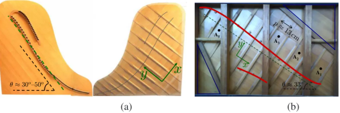
The piano soundboard (Fig. 1) is a large, almost plane, wood-structure. It includes a thin panel made out of glued spruce strips. A series of stiffeners – the ribs – are glued across the grain direction of the main panel’s wood. The ribs (also made of spruce, sometimes sugar pine) are only roughly equidistant. We define the x- direction as the grain direction of the panel and they-direction as that of the ribs.
On many pianos, one or two "cut-off" bars (in fir), much wider and thicker than the ribs, form, together with the sides of the soundboard, the so-called "cut-off corners".
Two maple bars – the bridges – thicker than the ribs, slightly curved, and eventually partly connected, are glued on the opposite face, roughly in the x-direction. The strings of the lower and the upper notes are attached to the (short) bass-bridge and to the main bridge, respectively. The soundboard of upright pianos is rectangular (the strings and the x-direction running diagonally). The soundboard of grand pianos looks like a backward slanted "L". The width of the soundboard is more or less 140 cm, corresponding to that of the keyboard. The height or length ranges from more or less 60 cm for very small uprights to more than 2 m for exceptionally large concert grands. The panel thickness isw≈8±2mm, the inter-rib distancep ranges from 10 to 18 cm in average (depending on pianos), and is slightly irregular from rib to rib.
Playing one note corresponds roughly to the following sequence of events: the pi- anist gives some kinetic energy to the hammer; the hammer escapes its mechanism and interacts very briefly (less than 5 ms) with one, two, or three unison strings; the strings vibrate and exert a localised force at the bridge of the soundboard, which makes the soundboard vibrating and radiating sound toward listeners. In the rest of this paper, "unison strings" will be shortened in "string".
A part of the initial kinetic energy of the hammer is very briefly given to the strings and then slowly transmitted to the soundboard and to the acoustical field. The spec- trum of one note (associated with a given pitch) includes a series of almost har- monically related partials: one partial consists of the slightly different modes of the strings and therefore, decays in time with a slow, complex pattern. For a given
∗ corresponding author
Email addresses:boutillon@lms.polytechnique.fr(Xavier Boutillon), kerem.ege@insa-lyon.fr(Kerem Ege).
y x
θ≈30o—50o θ≈33o
p≈ 13cm
y x
A1 A2 A3
A5
(a) (b)
Figure 1. (a): both sides of the soundboard of a grand piano.
(b): the rib side of the soundboard of the Atlas upright piano studied in [1], with the bridges superimposed as thick red lines and the locations of the accelerometers (in black). The grand soundboard had one cut-off bar, eventually removed. The upright soundboard in- clude one ribbed zone and two cut-off corners (blue-delimited lower-left and upper-right triangles).
note, the overall decay-time of each partial must not vary too widely between two consecutive partials. Musically, the timbre must also be balanced from note to note.
The main objective of this paper is to present a semi-analytical model of the sound- board from which one can predict the main characteristics of its vibration when it is excited by one string. More precisely, we focus on the vibration as seen by the string and by the acoustical field. The quantity that represents the coupling between the string and the soundboard is the point-mobility. According to Skudrzyk [2], the average of the real part of the point mobility is directly related to the modal density, which explains in part the emphasis on this parameter throughout the paper. The models presented here have no adjustment parameters and do not rely on the re- sults of dynamical experiments (except for the value of damping). They are meant to explore the changes in vibrational (and partly in radiative) overall properties of the soundboard or in string/soundboard coupling that would be induced by changes in wood characteristics or in the geometry of the various parts of the soundboard.
Compared to a finite-element model, our purpose is to provide more understanding and extreme numerical easiness, at the evident price of skipping details, both in space and partly in frequency.
We assume the following approximations:
• The soundboard represents a nearly fixed end for the string: strings and sound- board are dynamically weakly coupled and can therefore be modelled indepen- dently. In particular, it is considered that they have independent normal modes.
Therefore, after the end of the hammer-string interaction, each string vibrates on its normal modes and forces the vibration of the soundboard at frequencies that have no relationship with the soundboard eigenfrequencies.
• Effects due to the shell aspect and to the internal stress of the soundboard will be ignored.
• Only bending waves are considered in the soundboard and in its constituents (plates, bars), with motion in thez-direction.
• The mechanical function of the bridge where the string is attached (as seen by the string) is represented by a mechanical admittance, or point mobility:
ξ(ω) =˙ Y(ω)F(ω) (1) where F and ξ˙ are, in the Fourier domain, the force exerted by the string and the velocity of the soundboard. For a thin string, F and ξ˙ are vectors andY is a matrix. Only the vector components in the z-direction (normal to the plane of the soundboard) and the corresponding matrix coefficientYzz are considered.
The impedanceZQ(ω)analysed in Section 4 must be understood asZQ=Yzz−11.
• All structures (plates, bars) are considered as weakly dissipative, with damping values given by experiments or chosen arbitrarily.
In an experimental study [1], we analyse several features of the vibration of the soundboard of an upright piano in playing condition: linearity, modal dampings and modal frequencies up to 3 kHz, experimental modal shapes up to 500 Hz, boundary conditions, numerical modal shapes given by a finite-element modelling up to 3 kHz. As far as modal analyses are concerned, two experimental techniques were employed. At low frequencies, the soundboard was hit at 120 points on a rect- angular grid covering the whole soundboard and five accelerometers were installed as marked in Fig. 1-b. Results were obtained with a recent modal analysis tech- nique [4] based on parametric spectral analysis rather than FFT. Results are good up to about 500 Hz. Above this limit, the energy transmitted by the impact hammer to the structure is limited by either its weight (for light hammers) or by the duration of the impact which is ruled by the first returning impulse from the soundboard, in the order of magnitude of half the longest modal period. Another experimental technique had to be employed, namely to excite the soundboard by an acoustical field. The vibration was measured as before. Although the actual acoustical exci- tation was continuous in time, it was processed by deconvolution as to make use of the same modal parametric spectral analysis technique as before. However, only the modal frequencies and dampings could be reached by this technique but not the modal shapes. Since the excitation was not local, no point-mobility could be derived with this technique. In these experiments, the measurements are localised responses to the extended excitation by an acoustical field. The piano vibrating scheme of a piano is that of an extended response to a localised excitation. Since these situations are linked by physical reciprocity, results obtained in one situation are the same as in the other one.
1 By definition, Yzz isξ˙in response to a unit force Fz combined with zero-forces in the plane Oxy of the soundboard. Therefore, ZQ = Yzz−1 is different, in general, from Zzz which is the response force to a unit imposedξ˙and zero-velocity (that is: blocked motion) in theOxy plane. For a detailed discussion of differences between true mobility and true impedance measurements, see [3] for example.
Many observations can be summarised in Fig. 2, presenting the frequency depen- dency of the observed modal density, and in the following conclusions:
(1) The vibration is essentially linear.
(2) Except at very low frequencies, the boundary conditions are fixed.
(3) Below ≈1.1 kHz, the modes extend over the whole soundboard. The modal
density slowly increases and tends towards a constant value of about0.06modes Hz−1. The evaluation of the modal density is the same everywhere across the sound-
board.
(4) For frequencies above≈1.1 kHz, the ribs confine wave propagation and inter- rib spaces appear as structural wave-guides (wave-number selection in thex- direction), as already shown by Berthaut [5], § V.5. Moreover, modal shapes appear in Fig. 15 of [1] as localised in restricted areas of the soundboard, presumably due to the slightly irregular spacing and geometry of the ribs, in all pianos that we have observed. Localisation implies that the number of detected modes per frequency band may vary across the soundboard: at a given place anapparentmodal density is estimated. This phenomenon is further discussed at the beginning of Section 3.
(5) The loss factor is ≈ 2% ±1% over several kHz, without strong systematic variation.
In Section 2, devoted to the low-frequency regime, we model the ribbed part of the soundboard as a homogeneous plate and the whole soundboard as a set of sub- plates with clamped boundary conditions, and one bar representing the main bridge.
In Section 3, devoted to the high-frequency regime, we model the soundboard as a set of three structural wave-guides and also describe the transition with the sub- plate model. In Section 4, we derive the local mobility of the soundboard from the model. In Section 5, we analyse the implications of the model on the acoustical radiation and we discuss the consequences in terms of piano manufacturing.
102 103 10−2
10−1
Modal density (Hz−1 )
Frequency (Hz)
Figure 2. Modal densities observed on one piano soundboard (dots, data taken from [1]) and evaluated with the model proposed in this article (lines). The estimated values are the reciprocal of the moving average of six successive modal spacings, and reported at the mid-frequency of the whole interval.
Observed values at pointsA1(•),A2(N),A3(H), andA5(∗), whose locations are given in Fig. 1 (b). The choice for averaging explains why the first estimated point is well above the first detected mode of the soundboard, at 114 Hz.
Sub-plate model in the low-frequency regime (§ 2): gray lines.
: "Norway spruce". : "Sitka spruce".
: "Mediocre spruce" (see Table 1 for parameter values). Wave-guide(s) model in the high-frequency regime (§ 3), with Norway spruce parameters: colored lines.
Lower line : modal density of the (1,n)-modes in one single inter-rib space en- closing point A1 (see Eq. (18)); the horizontal line at the right hand-side of the figure corresponds to the asymptotic value of the modal density in this wave-guide, with all pos- sible(m, n)-modes.
Group of thin lines: modal density in the set of three adjacent wave-guides. : set of wave-guides in the vicinity ofA1; : vicinity ofA2.
: vicinity ofA3; : vicinity ofA5.
Thick line: transition between the three-waveguide model and the sub-plate model (§ 3.3), for pointA5.
2 Low-frequency behaviour: the sub-plate model
2.1 General presentation
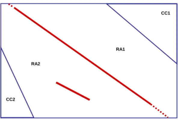
On almost all pianos, the main bridge extends throughout the entire soundboard and nearly reaches the rims. As shown in Fig. 3, we consider four zones of the sound- board: each side of the main bridge, with a fictitious extension up to the rim (ribbed areas RA1 and RA2) and the two cut-off corners (CC1 and CC2, unribbed except on some large grand pianos). On some pianos, mostly grands, only one or even no cut-off corner may exist. It is assumed that the cut-off bars and the main bridge are stiff and massive enough to keep modes nearly confined within one of these
CC1
CC2
RA1 RA2
Figure 3. Geometry of the subplates: cut-off corners (CC1 and CC2), ribbed areas of the soundboard (RA1 and RA2, the latter including the bass bridge). The main bridge is con- sidered as one of the sub-structures. The orthotropy angleθ⊥ (defined here as the angle between the keyboard-side of the soundboard and the main axis of orthotropy) is equal to −32.5o. The panel thickness and cut-off corners thickness are constant and equal to w=8mm.
regions. As discussed at the end of this section, this hypothesis is not fulfilled by the bridge, for the first modes. In the model proposed for the low-frequency regime (below≈1.1 kHz), the main bridge is also considered as a vibrating structure. The bass bridge is considered as adding mass to the ribbed area (being short and thick, its first eigenfrequency is relatively high). The dynamics of the cut-off bars is ig- nored. The main bridge and the different regions of the soundboard are considered as weakly coupled homogeneous structures. We tested the model by comparing the predicted and the measured modal densities. In the hypothesis of weakly coupled subsystems, the modal density of the soundboard n(f) is the sum of the modal densities of each structure considered separately ([6], Eq. (30), referring to [7], Chapter VI, §1.3):
n(f) =nmain bridge + nRA1 + nRA2 + nCC1 + nCC2 (2)
Given the hypotheses presented in Section 1, the plates that compose the piano soundboard are characterised by their surface densitiesµ=ρh=M/A(in generic terms), their rigiditiesD = Eh3
12(1−ν2) (idem) or dynamical rigidities D = D µ, their areas Aand their shapes and boundary conditions. As mentioned above, the surface density of RA2 includes the mass of the bass bridge: µRA2 = (MRA2 + Mbass bridge)/ARA2.
The cut-off corners are modelled as orthotropic plates (see Table 1 and Fig. 3 for the values of the parameters).
Each side of the main ribbed zone of the soundboard is considered as a homo- geneous orthotropic plate with similar mass, area, and boundary conditions. Ho- mogenisation is done according to Berthaut (Appendix of [8]), with values of the densities, elastic moduli, and principal Poisson’s ratios of the wood species given
EL(GPa) ER (GPa) GLR(GPa) νLR ρ(kg m−3)
"Sitka spruce" 11.5 0.47 0.5 0.3 392
"Mediocre wood" 8.8 0.35 0.4 0.3 400
"Norway spruce" 15.8 0.85 0.84 0.3 440
Fir 8.86 0.54 1.6 0.3 691
Maple 10 2.2 2.0 0.3 660
Table 1
Mechanical characteristics of spruce and fir species selected for piano soundboards. The data of the first and fourth lines are given by Berthaut [8] with methodology given in [5]
§ V.2.1, those of the second line by French piano maker Stephen Paulello, and the others by Haines [9]. The subscripts "L" and "R" stand for "longitudinal" and "radial" respectively.
The radial and longitudinal directions refer to how strips of wood are cut and correspond to the "along the grain" and the "across the grain" directions respectively.νLRis called the principal Poisson’s ratio.
In the geometry of the soundboard, thex- andy- directions correspond toLandRrespec- tively for the spruce panel:Ex=EL, Ey =ER, Gxy =GLR.
in Table 1. The choice for the values of the elastic constants and densities of the woods is discussed in § 2.3. Since the ribs are slightly irregularly spaced along the x-direction and have varying heights in they-direction, we adopt the approxima- tion that the flexibilities of the equivalent plate (inverse of rigidities) are the average flexibilities in each direction. In the piano that we have observed, the orthotropy ra- tioDHx/DyHof the homogenised plate is only≈1.4.
The frequency limit of the low-frequency regime is reached when the ribbed area of the soundboard cannot be considered as homogeneous. This occurs when the wavelength in the spruce panel (considered without ribs) becomes comparable to the inter-rib spacep. Given the generic dispersion equation Eq. (4) in an orthotropic plate, it comes:
ωgs = π p
!2
Dpanelx 1/2
(3) and the frequency limit of the regimeflim = min(fgs)is approximately 1.1 kHz.
2.2 Modal densities of the separate elements
In an orthotropic plate with thickness h, density ρ, Young’s moduli Ex and Ey, orthotropic angleθ⊥ 6= 0 (defined as the angle between the long side of the rect- angular plate and the main axis of orthotropy, see Fig. A.1), shear modulus Gxy, principal Poisson’s ratio νxy and modelled by the Kirchhoff-Love theory, the dis-
persion equation writes, in polar coordinates:
k4 hDx cos4(θ−θ⊥) + 2Dxy cos2(θ−θ⊥) sin2(θ−θ⊥) +Dy sin4(θ−θ⊥)i=ρ h ω2 (4) with:
Dx = Exh3
12(1−νxyνyx) Dxy = νyxExh3
12(1−νxyνyx)+ Gxyh3 6 Dy = Eyh3
12(1−νxyνyx) νyxEx =νxyEy
(5)
We adopt the following notations2 ζ =
sEx
Ey
=⇒ Dx
Dy
=ζ2 (6)
γ = Dxy
qDxDy
(7) α2 = 1
2 − Dxy
2qDxDy
= 1
2(1−γ) (8)
It is shown in the Appendix A that the asymptotic modal density of a rectangular orthotropic plate is independent of the orthotropy angleθ⊥:
n∞,orth = A π
sζ ρ h Dx
F(α) = A 2Dx
1/2
ζ1/2F(α)
F(0) = A 2Dx
1/4
Dy 1/4
F(α) F(0) (9) with F(α) =
Z π/2 0
1−α2sin2θ−1/2dθ (10)
We did not find in the literature an established formula for the low-frequency cor- rection accounting for the boundary conditions of an orthotropic plate with arbitrary θ⊥. Since it is a problem of practical importance (many modern materials are or- thotropic and modal analysis is applicable in the low-frequency range), we give a calculation of this correction in the Appendix A, for the case of a rectangular plate.
n(f) =n∞
1 + ǫL˜
q
4πAf
(11)
wheref =f n∞andL˜ are given by Eq. (A.16). As for an isotropic plate, the cor- rection is negative for constrained boundary conditions (ǫ =−1). For an arbitrary
2 ζ is the square root of the orthotropy ratio. γ is called the orthotropy parameter. The orthotropy is said elliptic whenγ = 1. For most materials[10],γis less than 1.
contour geometry, we propose Eq. (A.18) as a generalised expression of Eq. (A.16) forL.˜
The main bridge is modelled by a bar of lengthLb and dynamical rigidity Db, its modal density is independentnb(f)of the boundary conditions [11]:
nb(f) = Lb
Db 1/4
(2π f)1/2 (12)
2.3 Discussion
For a given geometry, the model presented above is predictive only if the density and elastic parameters of wood are known. This was not the case for the piano that we have analysed experimentally. In [1], we presented results of a finite-element model with various values for wood parameters. Even though the values of elastic parameters, on one hand, density on the other hand, may display large variations (say, up to 40%), the span of their ratio is much more restricted since, for a given species, denser comes along with stiffer. We present in Fig. 2 the modal densities predicted by Eq. (2) and the models derived above for the three sets of values indi- cated in Tab. 1. The values predicted by the model are systematically higher than those displayed by the FEM, which is to be expected since finite-element models have generally a stiffening bias.
As shown by the modal shapes displayed in Fig. 14 of [1], considering the main bridge as a separation between two zones of the soundboard is not a valid hypothe- sis for the very first modes but is acceptable as early as 250 Hz. Also, the boundary conditions for the very first modes are not fully constrained. Since assigning a nu- merical value to the modal density requires averaging, this concept is not applicable to the lowest modes anyway. Upper in frequency, some modes are confined to one side of the bridge whereas others extend on both sides, the bridge representing a nodal line. Therefore, the assumption of separate coupled plates might appear as not fully valid. However, weakly coupled plates or one plate including both yield almost the same asymptotic modal density sincen∞(f)is proportional to the sur- face of the plate. Only the low-frequency correction would differ since the overall perimeter is less than the sum of the two perimeters. The alternate model of a plate stiffened by a bar (the bridge) presented in Section 4, and others, also presented in [12], do not exhibit better matches with experimental results of the observed modal density in the low-frequency regime.
The influence on the modal density of the internal stress imposed to the sound- board by downbearing by the strings and constrained boundary conditions at the rim has not been modelled here. The FEM modelling presented in [1] showed that the magnitude of these effects is small, in the range of the approximations made in this paper. Including these effects in the model, presumably by an approximate
analytical approach, is left for future research.
3 High-frequency behaviour: coupled wave-guides
For frequencies above ≈1.1 kHz, mode counting yields different results depend- ing on the way modes are detected. As shown by numerical estimations of modes in Fig. 16 of [1], counting all the modes of the soundboard results in a modal density continuing the low-frequency trend. However, counting only the modes detected at one given point results in a modal density n(f) depending on the point where it is evaluated and decreasing with frequency. It must be noticed in Fig. 2 that the apparent abruptness in the fall of n(f) depends on how it has been estimated: if the average mean had been calculated over less than 6 modal spacings (≈120 Hz), the curve would have been less regular in general and the abruptness more pro- nounced. However, the main phenomenon responsible for the dependency ofn(f) on the point where it is evaluated is the localisation of modes in thex−direction, as shown in [1]. For non-localised modes (low-frequency regime), the vibration has the same order of magnitude everywhere, except in very restricted areas (nodes).
For localised modes (high-frequency regime), the amplitude of vibration outside the region of localisation decreases rapidly with distance (localised modes are as- sociated with evanescent waves). Therefore, the detection or the non-detection of a localised mode in a given point is much more robust to measurement conditions (exact position of the measuring device or excitation, signal-to-noise ratio, etc.) than it would be for an non-localised mode3. Altogether, the observations and as- sumptions presented above for the high-frequency regime seem reasonable enough to refer ton(f)astheapparent local modal density.
It is shown below that the confinement of the waves between ribs (wavenumber selection) together with localisation are responsible for the frequency dependency ofn(f)aboveflim. The vibration inside one wave-guide is described in § 3.1, the association of adjacent wave-guides is discussed in § 3.2 and a transition zone with the low-frequency regime is proposed in Section 3.3.
3.1 The wave-guide model
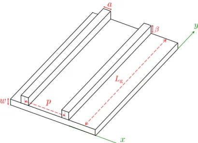
One inter-rib region, schematically represented in Fig. 4, behaves like an orthotropic plate of high aspect ratio, with special orthotropy. It is limited in width by the ribs and in length by the rim of the soundboard or by the cut-off bars. As a structure coupled to the rest of the plate, the rib should normally be considered with its
3 The non-detection of a non-localised mode requires that the measuring device be set exactly at a node. Additionally, the amplitude at the node depends strongly on damping.
Figure 4. Partial scheme of the soundboard between two successive ribs. The thickness of the spruce panel isw, the height of the rib isβ, the width of the rib isa.Lgis the average length of one inter-rib region (inter-rib spaces are not rectangular) and varies considerably among inter-rib spaces.
full dynamics, including rotation. It is assumed here that, above flim, the ribs are heavy enough to impose a nearly fixed condition to the bending transverse waves in the inter-rib region. Although this is true to a lesser extent, it is also assumed that torsion in the ribs do not influence significantly these bending waves. In other words, we assume that the dynamics of the ribs can be ignored and that they repre- sent hinged lines for the vibration in each inter-rib space. The propagation model is that of a structural wave-guide where transverse modes, with discrete wavenumbers kx,m =mπ
p, propagate in they-direction.
For a given kx,m, the dispersion law (4) in the orthotropic portion of the panel between two ribs becomes an equation onky only:
ky4+k2y 2Dxy Dy
kx,m2 +Dx
Dy
k4x,m− ρ h ω2 Dy
= 0 (13)
where theDi coefficients are given in Eqs. (5). Withkp = π
p and notations intro- duced in Eqs. 3, 6 and 7, it comes:
k4y + 2ζγ kx,m2 k2y + ζ2kx,m4 1− ω m2ωgs
!2
= 0 (14)
Introducing them-dependent normalisation relationships:
˜ky,m = ky
m kp
˜
ωm = ω
m2ωgs (15)
a dispersion equation of propagating waves in the wave-guide, identical for all transverse modes, is obtained:
˜k2y,m =ζqω˜2m − (1−γ2) − γ
(16)
Each angular frequencym2ωsgappears as low cut-off angular frequency associated with them-th transverse mode propagating in the wave-guide of widthp. The dis- persion curves ky(f) for the two first propagating transverse modes m = 1 and m = 2of an inter-rib space withp= 13cm are represented in Fig. 8. They differ noticeably from the succession of pass-bands (separated by stop-bands) that is ob- served in a more general treatment of the dynamics of the ribbed panel (see [13]
for example).
In the piano soundboard, the wavenumbersky,n (in the y-direction, parallel to the ribs) are determined by the lengthLg of the wave-guide and by the boundary con- ditions at the soundboard rim or at the cut-off bars. The ribs defining an inter-rib space have not the same lengths. We assume clamped boundary conditions (as in Section 2) and take forLg the length of the longest rib. The wavenumbersky,n are thus approximated byn+1
2
π
Lg with n∈N∗. The modal density in the wave- guide, defined as the reciprocal of the interval between two successive modal fre- quencies, can be estimated analytically by the usual method, briefly outlined below.
For a givenkx =m kp, the(m, y)-modes with angular frequency less than a given valueω⋆, have the eigen-wavenumbers less than k⋆y, given as a function ofω⋆ by Eqs. (15) and (16). In theky-space, these modes occupy the length|ky⋆|. Since each mode occupies a segment of length π
Lg, there areN⋆ =ky⋆Lg/πsuch modes. Dif- ferentiating with regard to the frequency yields the modal density:
nm(f) = ∆N
∆f = dN⋆
dky⋆ 2πdky⋆
dω⋆ = 2Lgdky
dk˜y
d˜ω dω
dk˜y
dω˜ (17)
= Lgp πDx
1/2
f˜m
m
qf˜m
2 −(1−γ2)
ζ
qf˜m
2 −(1−γ2) −γ
1/2
(18)
wheref˜m = f m2fgs.
For the first transverse mode (m = 1), the theoretical modal density of one of the wave-guides is reported in Fig. 2 (lowest solid thin blue line).
As frequency increases, transverse modes corresponding to all possible values of
mgradually appear in the wave-guide:
n(f) = Lgp πDx
1/2 +∞
X
m=1
f˜mH( ˜fm−1) mqf˜m2 −(1−γ2)
ζ
qf˜m2 −(1−γ2) −γ
1/2
(19) whereH(u)is the Heaviside function. However, since the second transverse mode appears above≈4.4 kHz, no jump in n(f)appears in Fig. 2. Those will be seen in the next sections, devoted to the synthesis of the mobility and to the acoustical radiation scheme.
Asymptotically, the modal density of the wave-guide, with all propagating trans- verse modes, is that of a narrow orthotropic plate of width p and length Lg (see Eq. (9) withA=p Lg), represented as an horizontal line at the right of Fig. 2.
3.2 Discussion
If the ribs were regularly spaced, the waves (with discrete values of kx) would extend throughout the entire soundboard and the observed modal density would be the same everywhere. As discussed above, irregular spacing is a very probable cause for modal localisation. Inspired by Anderson’s theory of (weak) localisation in condensed matter systems, the localisation of vibration in irregular mechanical structures has been extensively studied: see [14] for an introduction. We did not find established theoretical means for predicting the localisation areas in the piano soundboard but there is no theoretical reason either for restricting the vibration to one structural wave-guide. Moreover, the shapes of the localised modes reported in Fig. 15 of [1] show that they extend over more than one, but only a very few inter-rib spaces. Following a remark made earlier on the fast spatial attenuation of localised modes, we propose a simplified model in which the vibration extends over three adjacent wave-guides, as represented in Fig. 5. This assumption is also consistent with the fact that bending waves in adjacent wave-guides are coupled by the finite impedance of bending waves in ribs, particularly near the rim where the ribs are lower (smallerβ).
Altogether, we consider that (a) modes are mainly located in one wave-guide and selected according to the dimensions of this each wave-guide, (b) they have a con- tribution in the two adjacent wave-guides, (c) more remote regions can be con- sidered as quasi-nodal. When the whole soundboard vibrates under an acoustical excitation, one accelerometer must be sensitive, in this model, to the modes located in three wave-guides. The modal density observed at that point is the sum of the modal densities in each of the three wave-guides, as given by Eq. (19). As shown by Fig. 2, this simplification is in excellent accordance with the experimental re- sults above 1.5 kHz. One notices also that the model and the observations coincide on the differences between points. Moreover, multiplying the modal density in one
wave-guide by three (not represented in Fig. 2) would not give as a good fit with ob- servations as that obtained here by accounting for the fact that the two neighbouring wave-guides have different lengths.
Figure 5. Coupling between the bending waves (in the y-direction) in wave-guides sur- rounding the i-th one, as excited at Q, chosen here at the middle of the i-th wave-guide (widthpi). Wave-guides are separated by ribs (grey rectangles). When a forceFQis applied at pointQ, only thei−1-th, thei-th, and thei+ 1-th wave-guides are excited (see local- isation effect in text) and vibrate in their first transverse modekx,j = π
pj. The impedance Zj(ω)is the effect of the bending waves dynamics in thej-th wave-guide. Coupling results by the summation of the impedances (see text).
We analyse now the implications of the three-wave-guide model in terms of the mobility or impedance measured at one point, within the hypotheses and approxi- mations given in the Introduction. Mechanically, coupling between bending waves in the wave-guides operates via the transverse mode. By definition, an impedance Zj (considered here at the mid-line of wave-guide j) is created by the dynamics of the bending waves in thej-wave-guide (Fig. 5, see Section 4 for the analytical treatment). As a thought-experiment, cancelling the Young’s modulusEy (but not Ex) and the densityρin the central and right wave-guides would annihilate forces corresponding to these waves, thus cancellingZiandZi+1. In such a circumstance, imposing a motionξi,QatQwould still create the shape of the first transverse mode in the central wave-guide and thus create a motionξi−1, by coupling between the transverse modes aty = yQ; bending waves would therefore be generated in the left wave-guide. The force needed to establish the transverse mode in the central wave-guide is purely static and the corresponding impedance Zi,Ey=0 can be ne- glected above ωgs. Assuming perfect coupling and Q at the centre of the central wave-guide, the impedanceZQ would then beZi−1. In turn, these waves in wave- guidei−1would induce a motion in the central wave-guide, opposite to the motion in the left wave-guide. In normal circumstances (finiteEy andρ), it follows that the
impedance created atQis
ZQ=
i+1
X
j=i−1
Zj (20)
The sort of independence between the dynamics in thex-direction (dealing with the transverse modekx = π
p and its extension in the two adjacent wave-guides only) and in they-direction (propagation of bending waves in one wave-guide) explains the somewhat unusual circumstance in which modal motions and local forces add, yielding the addition of the modal mobilities inside a wave-guide (see Section 4) and the addition of wave-guide impedances.
Apparently, the three-waveguide model cannot account for the observed situation of sympathetic strings: playing a low note excites strings of a higher note (with its damper up) having common partials with the low note (usually, the fundamental of the high note). However, this situation implies a number of phenomena that are not examined in this paper. In the sympathetic strings situation, the vibration of the soundboard is forced at frequencies defined by the string(s), therefore combining several modal shapes. In particular, a low-frequency mode (that is: with a low value of the eigenfrequency) does respond, although weakly, to a high frequency excita- tion and can therefore excite a remote string. Another important feature is probably that modal dampings are much lower for string modes than for soundboard modes.
Finally, it must be noticed that the coupling of remote strings occurs via the motion of the main bridge. In the model, its transverse motion is considered as small com- pared to that of the rest of the soundboard but some significant torsion may well occur. In turn, parametric excitation of transverse string waves by the slight vari- ations in string tension induced by the motion of the bridge in the string direction may also play a role in the generation of the sympathetic strings effect.
3.3 Transition between the plate and the wave-guide models
Between 1 and 1.5 kHz, a more elaborate model taking into account the dynamics of the ribs would be necessary in order to describe the transition between the sub-plate and the 3-wave-guides models. We present here a cruder description. As explained at the end of § 2.1, the sub-plate model breaks atflim(the smallest offgs), given by Eq. (3)), defining the same upper bound of the sub-plate model for all measured points. We define the centre of the transition zone (noted by a double grey arrow in Fig. 2) as the frequency for which the sub-plate model and the three-waveguide model have the same modal density (e.g., at≈1310Hz for pointA5, as shown by the intersection of the corresponding modal density curves in Fig. 2). This supposed
"centre" also defines, somewhat arbitrarily, the upper bound of the transition zone.
Starting at the upper bound of the transition zone (where the wave-guide model
becomes fully valid) and decreasing frequency, the modes are expected to extend gradually throughout the soundboard. Guided by the experimental results, we can expect that this makes the region of the central wave-guide more remote, and there- fore, more nodal (for modes located in remote wave-guides) than when modes are localised in the adjacent wave-guides. In consequence, the modal density should be less than what it would be if the model was still holding. Arbitrarily, we consider that the modal density keeps the same value as the frequency decreases, down to the frequency at which the modal density of the single central wave-guide is reached.
From there, we took a linear transition toward the lower bound of the transition zone (upper bound of the sub-plate model), atfgs. The transition is represented by the thick plain broken line in Fig. 2.
4 Synthesised mechanical mobility and comparison with published measure- ments
In this section, we evaluate the point mobility at different points of the soundboard.
The point mobility at the bridge, where a string is attached, describes the coupling between the string and the soundboard. It is a key point for numerical sound syn- thesis based on physical models and more generally, for the understanding of sound characteristics: crucial musical parameters such as the damping of coupled string modes depend on the mechanical mobility and on the mistuning between unison strings [15]. In very generic terms, the modal density involves a ratio between mass and stiffness whereas mobilities involve their product. A good model should therefore be able to predict both.
Under the assumptions presented in Section 1, the mobilityYQat a pointQ(xQ, yQ) of the soundboard can be expressed as the sum of the mobility of the normal modes, considered as generalised coordinates, each having the dynamics of a linear damped oscillator4:
YQ(ω) = ξ˙Q(ω) FQ(ω) =jω
+∞
X
ν=1
ξν,Q 2
mν(ω2ν+jηνωνω−ω2) (21) wheremν is the modal mass,ην the modal loss factor,ων the modal angular fre- quency,ξQthe transverse displacement atQ, andξν,Qthe normalised displacement atQfor the modeν(modal shape). In this article, the modal mass is defined as the mass that gives the same maximum kinetic energy to the harmonic modal oscillator as that of the actual plate when both vibrate at the corresponding modal frequency with a unit maximum displacement.
With a modal density of roughly 0.02 Hz−1, about 200 modes are potentially in-
4 The convention for time-dependency isexp(jωt).
volved in the [0,10] kHz frequency range. The modal description does not bear any musical significance in itself and it is hard to think of cues that would help to sort out this huge number of modal parameters or to establish a hierarchy between them. If the quality of a piano was depending on the particular geometry of (some) modal shapes or on the particular values of (some) modal frequencies, those would be adjusted by piano makers. This is not the case, except perhaps at very particular locations like string-crossing, bridge ends or where the number of unison strings changes. Therefore, it seems reasonable to derive the values of the modal parame- ters from physical models, which depend on a much smaller number of parameters.
We present a mode-by-mode synthesis (§ 4.1) and a mean-value approach (§ 4.2) based on Skudrzyk’s theory [2].
We are not interested here in specific point-locations. Modal shapes can thus be described by random distributions:
Plate: ξν,Q = sin 2πα sin 2πβ
Wave-guide: ξν,Q = sin(2πkx,mxQ) sin 2πβ
(22) where the random quantities α and β are uniformly distributed in [0,1]. For Q near the centre of a waveguide,sin(2πkx,mxQ)is approximately 1 form odd and approximately 0 for m even. With the chosen definition of the modal mass and normalisation of modal shapes, it follows that all modal masses, whether for a plate or a wave-guide, are given bymν =Mplate,waveguide/4.
4.1 Synthesised mobility at the bridge
In the model described in Section 3, the main bridge is considered as a nodal line for most modes of the rest of the soundboard. Therefore, no sensible value ofξν,Q
can be assigned for these modes whenQis on the bridge. We follow an other ap- proximate model given by Skudrzyk [2, p. 1129, second approximation presented]
for a plate stiffened by a bar:
• The impedance of the soundboard at the bridge is the sum of the impedance of the bridge, considered as a beam (see next points below for its characteristics), and that of the central zone of the soundboard, considered as a plate (idem).
• The coupling between the bridge and the plate is described by a modified modal density of the bridge and by an added stiffness on the plate.
• The modified modal density of the bridge is obtained by adding to the bridge the mass of the plate.
• In its direction, the bridge imposes its stiffness to the plate (modified orthotropy compared to § 2.1, taken arbitrarily as elliptic).
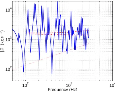
A synthesised impedance (reciprocal of the point-mobility) at the bridge is pre- sented in Fig. 6, according to Eqs. (21) and (22).
102 103 104
102 103 104
Frequency (Hz)
|Z|(kg.s−1)
Figure 6. Synthesised impedance at the bridge (blue solid line) and characteristic impedances (red lines, see § 4.2).
Dashed line: characteristic impedance of the soundboard Zc = 1/Yc, resulting from the sum of the characteristic impedances of the ribbed zone and of the bridge.
Dash-dotted line: characteristic impedance of the ribbed zone of the soundboard, with a stiffness in the bridge direction imposed by the bridge (see text).
Dotted line: characteristic impedance of the bridge considered as a beam mass-loaded by the plate (see text).
The first two values of the modal frequencies are those measured experimentally (114 and 134 Hz) but any physically reasonable choice would be acceptable since we are not interested in specific modal values. Beyond homogenisation that has been done in the low-frequency regime, a significant degree of irregularity re- mains in the soundboard, which must be considered here as uncertainty. According to [16], the spacing of the modal frequencies obeys a Rayleigh distribution instead of the Poisson distribution which rules modal spacings of regular structures. The values of the modal frequencies are determined by the random distribution and the modal density given by the model presented in Section 3:
fν+1 = fν+ 1
n(fν)r (23)
whereris a random number with the following probability distrubtion:
pd(x) = π x
2 exp −π x2 4
!
(24)
of mean 1 and variance 4
π −1. The same randomisation of the modal spacing was chosen by Woodhouse [17] for his statistical guitar5. WhenQis outside the cut-off corners, it must be considered as a node for the modes of the cut-off corners: the modal density in Eq. (23)) is restricted to that of the ribbed zone of the soundboard.
The modal frequencies of the bridge have not been randomised.
In accordance with the experimental values that have been found for the loss fac- tor [1], we attribute the following values to the modal dampings:
ην = αν
π fν = 2.3
100r (25)
whereri a random number following a chi-square probability distribution, as pro- posed by Burkhardt and Weaver [18, Eq. 8].
As long as the wavelength in the bridge is large compared to the inter-rib spacing, the bridge is coupled to the whole soundboard and the effect of localisation is ex- pected to be lost. It is expected to reappear when the half-wavelength in the bridge becomes equal to the inter-rib spacing. We have limited the frequency range of the synthesis to this limit.
4.2 Comparison with experiments: the mean-value approach
The only reliable and well-documented point-mobility measurements of a piano soundboard available in the literature are those by Giordano [19]. This author presents his measurements in the form of impedances. Giordano’s soundboard dif- fers in size from ours by only a few centimetres. We form the hypothesis that these pianos are dynamically comparable. This hypothesis is grounded by the observation that different pianos that have been measured in the literature seem to display com- parable equivalent isotropic rigidities (see Appendix B). A one-by-one comparison between modes, peaks, etc. between two pianos would be meaningless. We have adopted the mean-value approach of Skudrzyk [2]. His theory predicts the value of the geometrical mean of the real part of the mobility of a weakly dissipative struc- ture as a function of the modal density and the mass of the structure. It also shows that weak damping has no influence on the average level of the mobility. An outline and the main results are given below.
For a given mode, the geometrical mean ofℜ(YQ(ω))is:
Gν = n(f) 4Mν
with Mν = M < ξν2 >
ξν,Q2 (26)
5 See Eq. 5, where it seems that(2/π)has been written instead of(2/π)1/2.
whereM is the total mass of the structure.
For a plate or a beam, averaging on the modal shape and then on the modes yields the real part of the so-called characteristic mobility:
Gc,plate,beam = n 4Mplate,beam
. The geometrical mean of the imaginary part of the mobility differs between plates and beams. Finally, the characteristic mobilities are:
Yc,plate(f) = nplate(f)
4Mplate Yc,beam(f) = nbeam(f)
4Mbeam (1 − j) (27) In a waveguide, averaging on the modal shapes yields a different result:
Gc,guide,m = ǫQ,m
nguide
2Mg
, where, as shown above,ǫQ,mis shared by all modes corre- sponding to a given propagating transverse mode and depends on the location of Q. Near the middle of the wave-guide,ǫQ,mis approximately 1 for odd values ofm and approximately 0 for even values ofm. All the dispersion branches in the wave- guide (corresponding to the successivem-th propagating transverse modes) behave asymptotically like the dispersion equation of a beam (see Eq. (16) and Fig. 8). We consider therefore that Bc,guide ≈ −Gc,guide. Accounting for the coupling of three wave-guides described by Eq. (20), it comes:
1
Yc,3guides(f) =
3
X
k=1
X
m=1,2,...
nguide,k(f)
2Mguide,k (1 − j)ǫQ,m
−1
(28)
At the bridge, the characteristic impedances (reciprocal of the mobilities given by Eq. (27)) add, for the beam and plate modified as described in § 4.1. They are represented in Fig. 6 and their sum is reported in the left frame of Fig. 7, taken from Giordano.
Far from the bridge (right frame of Fig. 7), the characteristic mobility was computed according to Eq. (27) for the low-frequency regime and to Eq. (28) for the high- frequency regime, at a point similar to point "X" in Giordano’s piano (see Fig. 1 (a) in [19]). The low-to-high transition for the modal density is described in § 3.3. At the high-frequency end, the contribution of the second propagating transverse mode is somewhat arbitrary since the precise location along thex-axis is unknown.
Given the approximations made in the models and their application to a piano that we did not measure directly, one may consider that the match is striking, except in the transition zone, as could be expected. The excellent agreement in the upper frequency range may be considered as a partial confirmation of the coupling scheme devised in Section 3.2. Above the frequency for which half of the wavelength in the
bridge becomes comparable to the inter-rib spacing (≈3 kHz), the bridge begins to "see" the ribs. This might be an explanation for the impedance decrease at the bridge, above 3 kHz (left frame of Fig. 7). Again, irregular spacing is likely to cause localisation, coming along with a decrease in impedance (right frame of Fig. 7, above≈1 kHz.
Figure 7. Magnitude of measured point-impedances by Giordano[19] (solid black lines) and characteristic impedances modeled on a similar piano (dashed red lines, see text). Left frame: at the bridge, where strings C4 are attached. Right frame: far from the bridge, be- tween two ribs ("X"point in Fig. 1 (a) of [19]).
5 Some features of the acoustical radiation
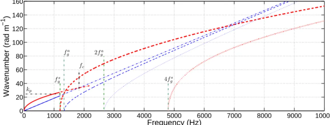
In this section, we examine how the soundboard acoustical radiation differs from the standard radiation scheme of a plain plate with the aim of examining some allegedly critical factors in piano making. For the sake of simplicity, we restrict our attention to the dispersion equations. Acoustical and structural waveumbers are denoted with "a" and "s" superscripts respectively.
5.1 Radiation regimes
Waves in a plate radiate efficiently (that is: far from the plate plane) when their wavelength is larger than that in air (supersonic waves). For structural waves prop- agating in a direction with a dynamical rigidity D, this occurs at a frequency f = c2a
2πD1/2. For an orthotropic plate, the transition from the subsonic to the su- personic regime is gradual, beginning at the frequency corresponding to the larger rigidity. For the values of the spruce parameters adopted above, the dynamical rigidities are larger in the x-directions: ≈150 in spruce plates (cut-off corners, usually ribless) and 100 m4s−2 in the homogenised central zone. The coincidence frequencies are 1.5 and 1.8 kHz respectively, both above the upper limit of the
low-frequency regime. In this regime, the soundboard behaves therefore like a set of plates in their subsonic regime (analysed in [20], for example). For the ho- mogenised ribbed zone of the soundboard (main area of acoustical radiation), the lowest of the dispersion curves is represented in Fig. 8 (thick solid red line), with fcdefined as the lowest frequency corresponding to coincidence in this orthotropic plate:
fc = c2a 2πDxH1/2
(29)
Abovefgs, the soundboard vibrates similarly to a set of three adjacent wave-guides.
We suppose that the rest of the soundboard is at rest, more or less ensuring a baf- fle for the acoustical field. Acoustical radiation by ribbed panels has been studied extensively since the 60’s and 70’s by Heckl, Maidanik, Mead, Mace, and many others since. With regularly spaced ribs, the vibration extends all over the plane.
The localised modal shapes are not known with precision in thex-direction but in any case, their spatial spectrum in this direction is maximum (with a more or less strong peak) atkxs ≈ mπ
p .
The structure-borne and the air-borne waves have the same spatial spectra in thexy- plane. Imposing a stationary field in thex-direction (withkxa = mπ/p) yields the following dispersion equation for the acoustical planes waves radiated in a direction belonging to theyz-plane with wave numberkayz:
kayz2+ mπ p
!2
= ω2
c2a (30)
The first two dispersion branches (m = 1 and m = 2) are drawn in Fig. 8 (thin dashed and dotted blue curves). Defining
fga = ca
2p (31)
these dispersion branches intercept thex-axis at fga and 4fga. Their asymptots are the air dispersion lineka = 2π f /ca(thin dash-dot blue curve). Due to the breadth of thekxs,a-spectrum (corresponding to localisation), these curves must be considered as the mean-lines of dispersion bands.
The ky components of the spatial spectra are also equal. The far-field acoustical radiation in thez-direction exists only if|kaz|is positive. For waves propagating in they-direction (which are radiated by the structural waves in the wave-guides),|kya| must be less than|kayz|: this is the usual "supersonic condition" for the radiation of a structure-borne wave.
It is clear in Fig. 8 that the subsonic or supersonic nature of the structural waves
0 1000 2000 3000 4000 5000 6000 7000 8000 9000 10000 0
20 40 60 80 100 120 140 160
Frequency (Hz) Wavenumber (rad m−1 )
2fga
fgs 4fgs
kp
fga fc
Figure 8. Dispersion curves of structural and acoustical waves generated inside and ra- diating outside the piano soundboard: supersonicvs.subsonic structural waves. Thick red curves: bending waves in the homogenised plate equivalent to the ribbed zone of the sound- board and in a structural wave-guides. Thin blue curves: corresponding radiated acoustical waves. The acoustical radiation is efficient (supersonic waves) for frequencies at which a blue curve is above the red curve with the same motive.
and : |ksx(f)|for the fastest bending waves (x-direction, lowest fc) in the homogenised plate equivalent to the ribbed zone of the soundboard, respectively below and abovefgs(crossing the dispersion line of plane waves in air atfc).
: |ksy(f)| for bending waves in the wave-guide between the second and third ribs for the first transverse mode of the guide, starting atfgs (see Eqs. 3 and 16).
:|ksy(f)|for bending waves in the wave-guide between the second and third ribs for the second transverse mode, starting at4fgs.
and : |ka(f)|for plane waves in air, respectively below and be- yondfgs(also the asymptot of the other dispersion curves in air). :|kayz(f)|for acoustical waves radiated by the main spatial componentkx =kp of the first propagating transverse mode in the wave-guides, starting atfga(see Eqs. 31 and 30).
: |kyza (f)| for acoustical waves radiated by the main spatial component kx = 2kp of the second propagating transverse mode in the wave-guides, starting at2fga.
depends on the relative values offga (given by Eq. (31) and fgs (given by Eq. (3)).
We examine now what is the condition on f for the structure-borne wave to be supersonic. With the following notations and normalisations (identical to Eq. (15) only form= 1):
K˜ = k kp
!2
Ω =˜ ω ωgs
!2
(32) the dispersion curves Eqs. (16) and (30), respectively in wave-guides and air, are transformed into:
K˜ys =ζ
qΩ˜ − m4(1−γ2) − m2ζ γ (33) K˜yza = Ω˜
Ω˜ag − m2 (34)
![Figure 2. Modal densities observed on one piano soundboard (dots, data taken from [1]) and evaluated with the model proposed in this article (lines)](https://thumb-eu.123doks.com/thumbv2/1bibliocom/473045.76019/7.892.136.730.111.370/figure-modal-densities-observed-soundboard-evaluated-proposed-article.webp)

![Figure 7. Magnitude of measured point-impedances by Giordano[19] (solid black lines) and characteristic impedances modeled on a similar piano (dashed red lines, see text)](https://thumb-eu.123doks.com/thumbv2/1bibliocom/473045.76019/23.892.145.727.203.455/figure-magnitude-measured-impedances-giordano-characteristic-impedances-modeled.webp)