HAL Id: hal-00785072
https://hal.archives-ouvertes.fr/hal-00785072
Submitted on 5 Feb 2013
HAL is a multi-disciplinary open access archive for the deposit and dissemination of sci- entific research documents, whether they are pub-
L’archive ouverte pluridisciplinaire HAL, est destinée au dépôt et à la diffusion de documents scientifiques de niveau recherche, publiés ou non,
Vietoris-Rips Complexes also Provide Topologically Correct Reconstructions of Sampled Shapes
Dominique Attali, André Lieutier, David Salinas
To cite this version:
Dominique Attali, André Lieutier, David Salinas. Vietoris-Rips Complexes also Provide Topologically Correct Reconstructions of Sampled Shapes. Computational Geometry, Elsevier, 2012, 46 (4), pp.448- 465. �10.1016/j.comgeo.2012.02.009�. �hal-00785072�
Vietoris-Rips Complexes also Provide Topologically Correct Reconstructions of Sampled Shapes
IDominique Attalia,∗, André Lieutierb,∗, David Salinasa,∗
aGipsa-lab, Grenoble, France
bDassault Système, Aix-en-Provence, France
Abstract
Given a point set that samples a shape, we formulate conditions under which the Rips complex of the point set at some scale reflects the homotopy type of the shape. For this, we associate with each compact set X of Rn two real-valued functions cX and hX defined on R+ which provide two measures of how much the set X fails to be convex at a given scale. First, we show that, when P is a finite point set, an upper bound on cP(t) entails that the Rips complex of P at scale r collapses to the Čech complex of P at scale r for some suitable values of the parameters t and r. Second, we prove that, when P samples a compact set X, an upper bound on hX over some interval guarantees a topologically correct reconstruction of the shape X either with a Čech complex ofP or with a Rips complex ofP. Regarding the reconstruction with Čech complexes, our work compares well with previous approaches when X is a smooth set and surprisingly enough, even improves constants when X has a positiveµ-reach. Most importantly, our work shows that Rips complexes can also be used to provide shape reconstructions having the correct homotopy type. This may be of some computational interest in high dimensions.
Keywords: Shape reconstruction, Rips complexes, clique complexes, Čech complexes, homotopy equivalence, collapses, high dimensions.
IThis work is partially supported by ANR ProjectGIGAANR-09-BLAN-0331-01.
∗Corresponding author
Email addresses: [email protected](Dominique Attali),[email protected](André Lieutier),
[email protected](David Salinas)
1. Introduction
In this paper, we formulate conditions under which the Rips complex of a point set reflects the homotopy type of the shape that the points sample using measures of how far this shape is from being convex.
Motivation. The problem of reconstructing shapes from point clouds arises in many fields, including computer graphics and machine learning [3, 23].
Maybe one of the simplest reconstruction method is to output an α-offset of the sample points, that is, the union of balls centered at the sample with radiusα. Assuming the shape is a smooth manifold [34, 19] or more generally has a positive µ-reach [17], it has been proved that this method provides indeed an approximation with the correct homotopy type for a sufficiently dense sample and a suitable value of the offset parameter α. Topologically, this is equivalent to computing the α-shape [24, 26] of the sample points, which can be obtained by first building the Delaunay triangulation and then keeping simplices that fit in an empty ball of radius α or less.
This approach works well for point clouds in three-dimensional space which have Delaunay triangulations of affordable size [5, 6]. But, as the dimension of the ambient space increases, the size of the Delaunay triangu- lation explodes [1] and other strategies must be found. If the data points lie on a low-dimensional submanifold, it seems reasonable to ask that the result of the reconstruction depends only upon the intrinsic dimension of the data.
This motivated de Silva [21] to introduce witness complexes and Boissonnat and Ghosh [13] to definetangential Delaunay complexes. For medium dimen- sions, Boissonnat and al. [12] have modified the data structure representing the Delaunay complex and are able to manage complexes of reasonable size up to dimension six in practice. In particular, they avoid the explicit repre- sentation of all Delaunay simplices by storing only edges in what they call the Delaunay graph, an idea close to that of using Vietoris-Rips complexes developed in this paper.
Vietoris-Rips complexes. Given a point set P and a scale parameter α, the Vietoris-Rips complex is the simplicial complex whose simplices are subsets of points in P with diameter at most 2α. Rips complexes are examples of flag complexes, and as such enjoy the property that a subset of P belongs to the complex if and only if all its edges belong to the complex. In other words, Rips complexes are completely determined by the graph of their edges. This
compressed form of storage makes Rips complexes very appealing for compu- tations, at least in high dimensions. Recent results study their simplification through homotopy-preserving edge collapses [36, 37] and edge contractions [8]. However, the strategy of using Rips complexes makes sense only if they are able to reflect the topology of the shape that their vertices sample. A closely related family of simplicial complexes are Čech complexes. Specifi- cally, the Čech complex of P at scale α consists of all simplices spanned by points in P that fit in a ball of radius α. The Čech complex of P at scale α is homotopy equivalent to the α-offset of P and therefore also possesses the ability to reproduce the topology of the shape sampled by P. This property was used by Chazal and Oudot [20] to extract topological information on the shape from the Rips complex filtration, by interleaving it with the Čech complex filtration and using persistence topology.
The main contribution of this paper is to unveil a more direct relation- ship between the respective topologies of the Rips complex and the sampled shape. Specifically, we give conditions under which Rips complexes capture the topology of the shape. In a different setting, it has been proved in [30, 31]
that the Rips complex of a point set close enough to a Riemannian manifold for the Gromov-Hausdorff distance shares the homotopy type of the mani- fold. However, these results focus on smooth manifolds, consider the intrinsic Riemannian metric instead of the Euclidean ambient metric and are not ef- fective since they do not give explicit constants. Nevertheless, they suggest that Rips complexes could be used in practice to produce topologically cor- rect approximations of shapes. If the distances are measured using the ℓ∞ norm then the Rips complex of P at scale α is equal to the Čech complex of P at scale α and is also homotopy equivalent to the union of hypercubes of side length 2α centered at the points of P [14]. In this case the authors in [7] state conditions under which the Rips complex of P reproduces the ho- motopy type of the shape sampled byP. In this paper we suppose distances are measured using the Euclidean norm. Extensions to more general metric spaces will be evoked in the conclusion.
Partially related to our work, we should mention [15] which relates the fundamental group of a Rips complex and its shadow (see below) in dimension 2 and give counterexamples in higher dimensions.
Sampling conditions. In any case, it is necessary for a point cloud to be accurate and dense enough to reflect the topology of the shape it samples.
The quality of the sample is typically expressed in terms of Hausdorff distance
to the shape. Guaranteed reconstruction methods are generally accompanied by results of the following form: if the Hausdorff distance is smaller than some notion oftopological feature sizeof the shape, then the output is topologically correct. First sampling conditions were expressed in terms of the reach, which is the infimum of distances between points in the shape and points in its medial axis [4, 2, 11, 34, 19]. Unfortunately, the reach vanishes on sharp concave edges and therefore is not suitable for expressing sampling conditions for non-smooth manifolds or stratified objects. To deal with this problem, authors in [17] introduce a new characterization of the feature size, the µ-reach, which allows them to formulate sampling conditions for a large class of non-smooth compact subsets of Euclidean space.
In this work, we introduce two new measures of feature size, both called convexity defects. Roughly speaking, they measure how far an object is from being locally convex, in the same manner as curvature measures how far an object is from being locally flat. In Section 5, we use these measures to express sampling conditions first for the Čech complex and second for the Rips complex. Regarding the reconstruction with Čech complexes, our work compares well with previous approaches when X is a smooth set and surprisingly enough, even improve constants when X has a positive µ-reach.
Most importantly, this new framework allows us to prove that Rips complexes also provide topologically correct reconstruction, assuming shapes have a positive µ-reach, for µsufficiently large.
The remaining sections are organized as follows. In Section 2 we present the necessary background and define the Čech complex and the Rips complex.
In Section 3 we introduce and study our two convexity defects functions cX : R+ → R+ and hX : R+ → R+ that we associate with any non-empty bounded subset X ⊂Rn. Section 4 describes a condition based on cP under which the Rips complex of a point set P at scale α deformation retracts to the Čech complex of P at scale α. This key condition is encapsulated in Theorem 7. In Section 5 we consider a shapeXsampled by a point setP and formulate conditions under which either Čech complexes or Rips complexes of P provide approximations ofX with the correct homotopy type. We express those conditions first in terms of an upper bound on cX then for shapes with a positive µ-reach. Section 6 concludes the paper.
2. Background
In this section we introduce the basic definitions and properties needed in the paper and review two well-known examples of simplicial complexes:
the Čech complex and the Rips complex.
2.1. Metric space, distances, smallest enclosing ball
Throughout this paper, we shall consider subsets of the Euclidean n- space Rn for n ≥ 1. The Euclidean distance between two points x and y of Rn is denoted kx −yk. Given two subsets X and Y of Rn, we write dH(Y |X) = supy∈Y d(y, X) for the one-sided Hausdorff distance of Y from X, where d(y, X) is the infimum of the Euclidean distances between y and points x in X. Observe that dH(Y |X)≤ ε if and only if Y is contained in theε-offsetXε ={y∈Rn|d(y, X)≤ε}. TheHausdorff distancebetweenX and Y is dH(X, Y) = max{dH(X|Y), dH(Y |X)}. Recall that the diameter of a subset σ of Rn is the supremum of distances between pairs of points in σ, which we denote as Diam(σ) = supp,q∈σkp−qk. A subset σ is said to be bounded if its diameter is finite.
The closed ball with center z and radius r is denoted B(z, r). Balls will always be assumed to be closed, unless stated otherwise. It is well known that the smallest ball enclosing a non-empty bounded set σ of Rn is well-defined (see Appendix A for a proof). We denote its center by Center(σ) and its radius by Rad(σ). Writing Hull(X) for the convex hull of a subset X ⊂ Rn and X for the closure of X, it is not hard to check (by contradiction) that
Center(σ) ∈ Hull(σ).
The following inequalities will be useful in Section 2.4 for relating Čech and Rips complexes:
1
2Diam(σ) ≤ Rad(σ) ≤ ϑn
2 Diam(σ) where ϑn=
r 2n
n+ 1. (1) The right most inequality is also known as Jung’s Theorem and a short proof can be found in [22]. In particular, we have Rad(σ) < √12Diam(σ) for all dimensions n.
2.2. Abstract simplicial complexes
LetP be a finite set of points inRn. We call any non-empty subsetσ⊂P anabstract simplex. Itsdimensionis one less than its cardinality. Ai-simplex is an abstract simplex of dimension i. If τ ⊂ σ is a non-empty subset, we call τ a faceof σ and σ a cofaceof τ. An abstract simplicial complexK is a collection of non-empty abstract simplices that contains, with every simplex, the faces of that simplex. The vertex set of the abstract simplicial complex K is the union of its elements, Vert(K) = S
σ∈Kσ. A subcomplex of K is a simplicial complex L ⊂ K. A particular subcomplex is the i-skeleton consisting of all simplices of dimension i or less, which we denote by K(i). The shadow ofK is the subset of Rn covered by the convex hull of simplices in K, ShdK = S
σ∈KHull(σ), not to be confused with |K|, the underlying space of a geometric realization of K; see [33]. Let N be the cardinality of the vertex set of K. The underlying space |K| of K can be defined (up to a homeomorphism) by considering a map f : Vert(K) → RN−1 that sends the N vertices ofK toN affinely independent points inRN−1 and by setting
|K| = S
σ∈KHull(f(σ)). Generally, |K| and ShdK are not homeomorphic, as illustrated in Figure 1.
We now review two natural ways of constructing an abstract simplicial complex, given as input a finite set of points in Rn and a feature scale pa- rameter t ≥ 0. The definitions given below appear in different forms in the literature.
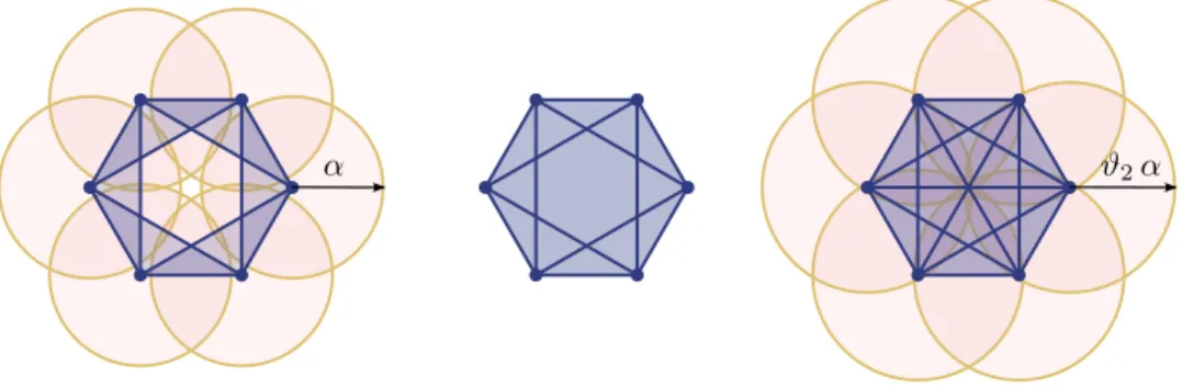
α ϑ2α
Figure 1: Left: the Čech complex with parameterαcomprises six triangles and is homo- topy equivalent to a circle. Middle: the Rips complex with parameterαcontains two more triangles and is homeomorphic to a 2-sphere. Its shadow is a topological disk. Right: the Čech complex with parameterϑ2αcontains all faces of the 5-simplex and is homeomorphic to a 5-ball.
2.3. The Čech complex
The Čech complex C(P, t) is the abstract simplicial complex whose k- simplices correspond to subsets of k+ 1 points that can be enclosed in a ball of radius t,
C(P, t) = {σ| ∅ 6=σ ⊂P,Rad(σ)≤t}.
Equivalently, a k-simplex {p0, . . . , pk} belongs to the Čech complex if and only if the k + 1 closed Euclidean balls B(pi, t) have non-empty common intersection. Let NrvF = {G ⊂ F | T
G 6= ∅} denote the nerve of the collectionF. The Čech complex is the nerve of the collection of balls{B(p, t)| p ∈ P}. Since balls are convex, the Nerve Lemma [10, 27] implies that the Čech complexC(P, t)is homotopy equivalent to the union of these balls, that is, |C(P, t)| ≃Pt=S
p∈P B(p, t).
2.4. The Rips complex
TheVietoris-Rips complexis a variant of the Čech complex which is easier to compute. The Vietoris-Rips complex, R(P, t) is the abstract simplicial complex whose k-simplices correspond to subsets of k+ 1 points in P with diameter at most 2t,
R(P, t) = {σ| ∅ 6=σ⊂P,Diam(σ)≤2t}.
For simplicity, we refer to R(P, t) as the Rips complex. Recall that the flag complex of a graph G, denoted FlagG, is the maximal simplicial complex whose 1-skeleton is G. The Rips complex is an example of a flag complex.
More precisely, this is the largest simplicial complex sharing with the Čech complex the same 1-skeleton, R(P, t) = Flag C(P, t)(1). Generally, R(P, t) and C(P, t) do not share the same topology; see Figure 1. It follows that the Rips complex R(P, t)is generally not homotopy equivalent to thet-offsetPt. Our goal in the next section is to find a condition on the point set P which guarantees that |R(P, t)| ≃ |C(P, t)| and therefore|R(P, t)| ≃Pt. Along the way, we will need a result in [22] which is a consequence of Equation (1) and which says that there is chain of inclusion
C(P, t) ⊂ R(P, t) ⊂ C(P, ϑnt) whereϑn=
r 2n
n+ 1. (2)
3. Convexity defects measures
In this section, we introduce and study two functions that one can as- sociate with any non-empty bounded subset X ⊂ Rn and that provide two different ways of measuring convexity defects of X. Based on the first func- tion, we will formulate in Section 4 a condition which suffices to guarantee that the Rips complex of a finite set of points P at scale α deformation re- tracts to the Čech complex of P at scale α. Based on the second function, we will formulate in Section 5 sampling conditions under which the Čech and Rips complexes of a point set P provide topologically correct reconstructions of a shape X sampled by the points in P.
3.1. Definitions and basic properties
To avoid lengthy sentences, we adopt the convention that the subsetX ⊂ Rn is always assumed to be non-empty and bounded in this section. In particular, any non-empty subset σ ⊂ X is also bounded and thus has a well-defined smallest enclosing ball. We first define the set of centers of X at scale t as the subset (see Figure 2, left):
Centers(X, t) = [
∅6=σ⊂X Rad(σ)≤t
{Center(σ)}.
Recalling that Hull(X) denotes the convex hull of X, we then extend the notion of convex hull. Specifically, we define the convex hull of X at scale t as the subset (see Figure 2, right)
Hull(X, t) = [
∅6=σ⊂X Rad(σ)≤t
Hull(σ).
IfX is compact thenHull(X, t)is a superset of Centers(X, t). IfP is a finite set of points then Hull(P, t) is the shadow of the Čech complex C(P, t).
Definition 1 (Convexity defects functions). Given a subset X ⊂ Rn, we associate to X two real-valued functions: the first one cX :R+ →R+ is defined by cX(t) =dH(Centers(X, t)|X) and the second one hX :R+ →R+
is defined by hX(t) = dH(Hull(X, t)|X).
Figure 2: Smallest offset of X containingCenters(X, t)on the left and Hull(X, t)on the right.
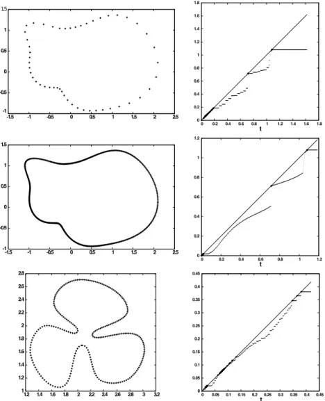
Intuitively, cX and hX can be thought of as functions that measure the convexity defects of X at a given scale. To make this idea precise, observe that if X ⊂ Rn is compact, then we have the three equivalences: X convex if and only if cX = 0 if and only if hX = 0. The two convexity functions cX and hX will play a different role. While cP is all we need to study the Rips complex of a finite point set P in Section 4, it turns out that hX is more stable than cX and will be used in Section 5.1 to express sampling conditions in reconstruction theorems. We plotted the graph of the function cP for various finite point sets in Figure 10.
Before studying in more details functions cX and hX in the next two sections, let us make some brief remarks. Because X is a subset of both Centers(X, t) andHull(X, t), it follows that the two one-sided Hausdorff dis- tancesdH(X|Centers(X, t))anddH(X| Hull(X, t))vanish. Hence, we could have used in the above definition two-sided Hausdorff distances instead of one-sided Hausdorff distances. The two functions cX and hX both vanish at 0, are increasing in the interval [0,Rad(X)] and become constant above Rad(X). Since Center(σ) ∈ Hull(σ), we have cX ≤ hX. It is easy to check that for a subsetX ⊂Rnand two non-negative real numberstandα, the fol- lowing three conditions are equivalent: (1) hX(t)≤ α; (2) Hull(X, t) ⊂Xα; (3) [Rad(σ) ≤ t =⇒ Hull(σ) ⊂ Xα] for all σ ⊂ X. In particular, we get that hX(t)≤ t for allt ≥ 0 since Rad(σ)≤ t =⇒ Hull(σ) ⊂σt as a direct consequence of Lemma 1 (below) applied for x=y.
Lemma 1. For any non-empty bounded subset σ ⊂ Rn, any point x ∈ Rn
and any point y ∈ Hull(σ), we have that d(x, σ)2 ≤ kx−yk2 + Rad(σ)2 − ky−Center(σ)k2.
B1
H01
σ
B0
y
Center(σ) x
Hull(σ)
Figure 3: Notation for the proof of Lemma 1.
Proof. Suppose d(x, σ) > kx − yk for otherwise the result is clear. Let B0 be the smallest ball enclosing σ and let B1 be the largest ball centered at x whose interior does not intersect σ; see Figure 3. By construction, σ ⊂ B0 \B1. Recall that the power distance of a point y from a ball B is πB(y) = ky−zk2 −r2, where z is the center of B and r its radius. Let H01 be the set of points whose power distance to B0 is at most as large as the power distance to B1. H01 is a closed half-space which contains the set difference B0 \B1. In particular, it contains σ and any point y ∈ Hull(σ).
Thus, πB0(y)≤πB1(y) and the result follows.
3.2. Characterizing critical values of the distance function
In the previous section we noted that cX(t) ≤ hX(t) ≤ t for all t. The goal of this section is to establish that equality is attained if and only if t is a critical value of the distance function toX. This property will not be used before Section 5 but sheds light on results of Section 4.
We need some definitions. The distance function d(·, X) to the com- pact set X ⊂ Rn maps every point y ∈ Rn to its Euclidean distance to X, d(y, X) = minx∈Xkx−yk. Although the distance function is not differ- entiable, it is possible to define a notion of critical points analogue to the
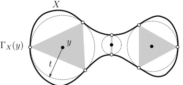
classical one for differentiable functions as illustrated in Figure 4. Specifi- cally, Grove defines in [29, page 360] critical points for the distance function to a closed subset of a Riemannian manifold. We recast this definition in our context as follows. Let ΓX(y) = {x ∈ X | d(y, X) = kx−yk} be the set of points in X closest to y:
Definition 2. We say thaty∈Rnis acritical pointof the distance function d(·, X) if y ∈ Hull(ΓX(y)). The critical values of d(·, X) are the images by d(·, X) of its critical points.
ΓX(y) y
t X
Figure 4: The black points are the critical points of the curve X.
Next lemma provides two characterizations of the critical values of the distance function to a compact set X ⊂ Rn, based respectively on the two convexity defects functions cX and hX.
Lemma 2. For any compact set X ⊂ Rn and any real number t > 0, the following three conditions are equivalent: (1) t is a critical value of d(·, X);
(2) cX(t) =t; (3) hX(t) = t.
Proof. Consider a non-empty bounded subset σ ⊂ Rn and a point y ∈ Rn. Makingx=yin Lemma 1, we observe that ify∈Hull(σ)satisfiesd(y, σ)≥t and Rad(σ)≤t, then y= Center(σ)and t = Rad(σ).
Let us prove that (1) =⇒ (2). Consider a critical pointywhose distance toX ist and set σ = ΓX(y)as shown in Figure 4. By definition y∈Hull(σ) and by construction d(y, σ) =t and Rad(σ)≤t. Thanks to our observation, it follows that y = Center(σ) and consequently cX(t) = t. The implication (2) =⇒ (3) follows from cX(t) ≤ hX(t) ≤ t. Let us prove that (3) =⇒ (1). In other words, suppose hX(t) = t and let us prove that t is a critical value of d(·, X). Since X is compact, hX(t) = t means that we can find
a compact set ∅ 6= σ ⊂ X with Rad(σ) ≤ t and y ∈ Hull(σ) such that t = d(y, X) ≤ d(y, σ). Our observation then implies that y = Center(σ), t = Rad(σ) and σ represents a set of points in X with minimum distance to y. Since y ∈ Hull(σ) ⊂ Hull(ΓX(y)), it follows that y is a critical point of the distance function to X, which concludes the proof.
An adaptation of Morse theory to distance functions tells us that changes in the topology of t-offsetsXtoccur when the offset parametert reaches crit- ical values of the distance function to X. Indeed, slightly recasting Proposi- tion 1.8 in [29, page 362], we have:
Theorem 3 (Isotopy Theorem [29]). Let X ⊂ Rn be a compact set and let β ≥ α > 0 be two real numbers. If the distance function d(·, X) has no critical values in the interval [α, β], then Xβ deformation retracts to Xα.
Our characterizations of critical values allow us to reexpress the condition in the above theorem. To be specific, we get that ifcX(t)< tfor allt∈[α, β], thenXβ deformation retracts toXα. ReplacingX by a finite point setP and using that the Čech complexC(P, t)is homotopy equivalent to thet-offsetPt, we obtain that C(P, β)is homotopy equivalent toC(P, α)whenevercP(t)< t for all t ∈ [α, β]. We shall see in Section 4 that under the same condition a stronger result holds, namely the existence of a sequence of collapses from C(P, β)toC(P, α). Strengthening this condition, we will be able to guarantee the existence of a sequence of collapses from R(P, β) to C(P, α). Variants of this condition will then be devised in Section 5 to ensure topologically correct reconstruction of shapes by Čech or Rips complexes.
3.3. Stability
In this section, we state the stability ofcX and hX. For technical reasons, we need the stability of cP under perturbations of P at the end of the proof of Theorem 7 in Section 4 to relax the assumption that the finite point setP that we consider is in general position. The stability ofhX under perturbation of X will be crucial for establishing reconstruction theorems in Section 5.
Lemma 4. For every pair of subsets X andY of Rn such thatdH(X, Y)≤ε and for every t≥0, we have
cY(t) ≤ cX(t+ε) +√
2tε+ε2+ε.
Proof. Consider a non-empty subset σ ⊂ Y with Rad(σ) ≤ t and set ξ = X ∩σε. By construction, ξ is non-empty and dH(ξ, σ) ≤ ε. Hence, setting δ = √
2tε+ε2, Lemma 16 implies that Rad(ξ) ≤ t+ε and kCenter(σ)− Center(ξ)k ≤δ. We get
Center(σ) ⊂ Center(ξ)δ ⊂ XcX(t+ε)+δ ⊂ YcX(t+ε)+δ+ε, yielding to the result.
Lemma 5. For every pair of subsetsX andP of Rn such thatdH(X, P)≤ε and for every t≥0, we have hP(t)≤hX(t+ε) + 2ε.
Proof. Consider a non-empty subset σ ⊂ P with Rad(σ) ≤ t and set ξ = X ∩σε. By construction, ξ is non-empty and dH(ξ, σ)≤ ε. Hence, Lemma 16 implies that Rad(ξ) ≤ t +ε. Using Hull(ξε) = Hull(ξ)ε, we get that Hull(σ)⊂Hull(ξ)ε ⊂XhX(t+ε)+ε ⊂PhX(t+ε)+2ε, yielding the result.
4. From Rips to Čech complexes
In this section, we introduce a 2-parameter family of Rips complexes and give the precise condition on a finite point set for which we can prove that a Rips complex in this family deformation retracts to a Čech complex.
We begin by defining this family of Rips complexes and state our results in Section 4.1. We then introduce the tools we need to prove our results in Section 4.2. The proofs are presented in Section 4.3.
4.1. Quasi Rips complexes and statement of results
Following [16], we first define a 2-parameter family that contains prior Rips complexes as a subfamily. The motivation for this construction is to account for the uncertainty of measures by allowing uncertainty of the edges belonging to Rips complexes in the family; see [16].
Definition 3. For any point set P ⊂ Rn and any real numbers α, β ≥ 0 with α ≤ β, we call the flag complex of any graph G satisfying R(P, α) ⊂ FlagG⊂ R(P, β)an (α, β)-quasi Rips complexof P.
In other words, the simplicial complex FlagG is an (α, β)-quasi Rips complex of P if and only if every pairs of points in P within distance 2α are connected by an edge in G and no edge of G has length larger than 2β.
Equivalently, for every pairs (p, q) ∈ P2, kp−qk ≤ 2α implies pq ∈ G and kp−qk>2βimpliespq 6∈G. In particular,Kis an(α, α)-quasi Rips complex of P if and only if K =R(P, α).
To state our results, it is convenient to defineαto be an inert value ofP if Rad(σ) 6=α for all non-empty subsets σ ⊂ P. The finiteness of P implies thatP has only finitely many non-inert values. Thus, assumingαto be inert is not a too restrictive hypothesis.
As a warm-up, we first state conditions in Theorem 6 (below) under which there exists a sequence of elementary collapses which transform one Čech complex into another one. We recall that anelementary collapseis the operation that removes a pair of simplices(σ, τ)from a simplicial complexK assuming τ is the unique proper coface of σ in K. The result is a simplicial complex K\ {σ, τ} to which K deformation retracts.
Theorem 6. Let P ⊂ Rn be a finite set of points. For any real numbers β ≥α≥0 such that α is an inert value of P and cP(t)< t for all t∈[α, β], there exists a sequence of elementary collapses from C(P, β) to C(P, α).
Theorem 6 can be thought of as a combinatorial version of the Isotopy theorem presented in Section 3.2. We are now ready to state our main theorem:
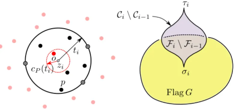
Theorem 7. Let P ⊂ Rn be a finite set of points. For any real numbers β ≥α≥0 such thatαis an inert value of P and cP(ϑnβ)<2α−ϑnβ, there exists a sequence of elementary collapses from any (α, β)-quasi Rips complex of P to the Čech complex C(P, α).
Note that choosing β = α in the theorem gives conditions under which
|R(P, α)| ≃ |C(P, α)| ≃ Pα. Figure 7 on the left provides a graphical repre- sentation of the hypothesis of the theorem. Let us sketch quickly the proof of Theorem 7. Observe that the condition cP(ϑnβ)<2α−ϑnβ implies that cP(t)< t for all t ∈[α, ϑnβ]since
cP(t) ≤ cP(ϑnβ) < 2α−ϑnβ ≤ α ≤ t,
whenever α≤t≤ϑnβ. Theorem 6 then implies that there exists a sequence of collapses reducing C(P, ϑnβ)toC(P, α). Since any (α, β)-quasi Rips com- plexFlagGis nested betweenC(P, α)andC(P, ϑnβ), the key idea in the proof of the above theorem is to monitor changes in the complex C(P, t)∩FlagG as we decrease the scale parameter t from ϑnβ to α, that is as we go from C(P, ϑnβ) toFlagG. The proof is given in Section 4.3. Before embarking in the proof, we will define collapses and extended collapses in the next section.
4.2. Extended collapses
In this section, we introduce collapses and extended collapses which will turn out to be convenient to describe changes that occur in the families of complexes that we consider in our proof of Theorem 7.
We need some definitions. The inclusion defines a partial order relation on simplices. Given a set of simplices Σ and a simplexσ∈Σ, we say thatσ is inclusion-maximal in Σ if σ has no proper coface in Σ. Similarly, we say that σ is inclusion-minimal if it has no proper face in Σ. When clear from the context we will omit Σ. Supposeσ is a simplex of the simplicial complex K. The star of σ in K, denoted StK(σ), is the collection of simplices of K havingσas a face. The closure ofStK(σ)is denotedStK(σ); it is the smallest simplicial complex containing StK(σ). The link of σ in K, denoted LkK(σ), is the collection of simplices ofK lying inStK(σ)that are disjoint from σ. A simplicial complex K is said to be a cone if it contains a vertex o such that the following implication holds: σ ∈ K =⇒ σ∪ {o} ∈ K. The vertex o is called the apexof the cone. By definition a cone can never be empty since it always contains at least its apex.
σ
o o
σ
γ γ
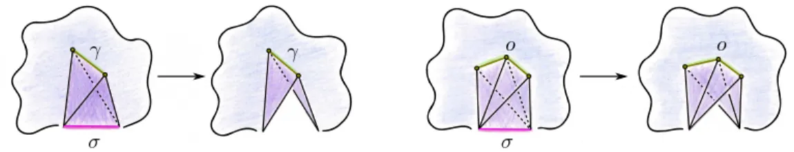
Figure 5: Left: In a classical collapse, the link ofσhas a unique inclusion-maximal simplex γ. Equivalently, the star ofσhas a unique inclusion-maximal simplexσ∪γdifferent from σ. Right: In an extended collapse, the link ofσis a cone with apex o.
Given a simplicial complex K, we are interested in the operation that removes the entire star of a simplex σ ∈ K as illustrated in Figure 8. Pro- vided that there is a unique inclusion-maximal simplex τ 6=σ in the star of σ, it is well-known that |K| deformation retracts to |K \StK(σ)| and the operation that removes StK(σ) is then called a collapse [25]. Any collapse can be decomposed into a finite sequence of elementary collapses. Follow- ing and extending what was done in [9], we call the operation that removes StK(σ)assuming the weaker condition that the link ofσis a cone anextended collapse. Our terminology finds its justification in the following lemma.
Lemma 8. Let K be a simplicial complex and letσ be a simplex of K. If the link ofσ is a cone, then there is a sequence of collapses fromK toK\StK(σ).
Proof. First, we establish that a cone Lcan always be reduced to its apex o by a sequence of collapses. Suppose L6={o}for otherwise the result is clear and consider an inclusion-maximal simplex in L. It has the form α ∪ {o} with o 6∈ α ∈ L. Let us prove that the operation that removes the pair of simplices (α, α∪ {o}) is a collapse. If β is a coface of α, then β∪ {o} is a coface of α∪ {o}. Sinceα∪ {o} is inclusion-maximal, the only possibility is that β ∪ {o} = α∪ {o}, showing that all cofaces of α are faces of α∪ {o}. Thus, removing the pair (α, α∪ {o}) is a collapse and the result is still a cone with apex o but with a smaller number of simplices. By repeating the process we eventually get a complex reduced to {o}.
Now, suppose the link of σ in K is a cone L with apex o. We deduce from the previous sequence of collapses that reduces L to {o} a sequence of collapses that reduces K to K \StK(σ) as follows. To each collapse that removes the pair (α, α∪ {o})inL described above, we associate the collapse that removes the pair(σ∪α, σ∪α∪ {o})inK. Indeed, since αhas a unique proper coface α∪ {o}in L, it follows that σ∪α has a unique proper coface σ∪α∪ {o} in K. At the end of this sequence of collapses, the link of σ is reduced to {o}. After a last collapse that removes the pair (σ, σ ∪ {o}) we get K\StK(σ).
4.3. Proof of results
We will prove directly Theorem 7 and omit the proof of Theorem 6 since one can easily derive a proof of Theorem 6 by slightly adapting the first part of the proof below.
Proof of Theorem 7. LetGbe a graph whose flag complex is an (α, β)-quasi Rips complex of P. For t ≥ 0, consider the simplicial complex F(t) = C(P, t)∩FlagG. Clearly, we have the chain of inclusions:
C(P, α) ⊂ R(P, α) ⊂ FlagG ⊂ R(P, β) ⊂ C(P, ϑnβ)
and therefore F(α) = C(P, α) and F(ϑnβ) = FlagG. As we continuously increase the feature parameter t from α to ϑnβ, we get a finite family of nested Čech complexes:
C(P, α) = C ⊂ C ⊂ · · · ⊂ C =C(P, ϑ β).
For 0 < i < k, let ti be the smallest value of t such that Ci = C(P, t) and set Fi = F(ti). In particular, Ci = C(P, ti) and Fi = Ci ∩FlagG.
Correspondingly, we get a 1-parameter family of simplicial complexes by intersecting each complex Ci in the above sequence with FlagG:
C(P, α) =F0 ⊂ F1 ⊂ · · · ⊂ Fk= FlagG.
Let us first assume that P satisfies the two generic conditions (⋆) and (⋆⋆) instead of the condition that Rad(σ)6=α for all non-empty subsetsσ ⊂P:
(⋆) For all simplices σ, τ ⊂ P, if Rad(σ) = Rad(τ) then Center(σ) = Center(τ);
(⋆⋆) For any ballB, the set of simplices inP that have B as a smallest en- closing ball is either empty or has a unique inclusion-minimal element.
Under these two conditions, we prove the theorem in two stages. First, we show that Ci−1 is a collapse of Ci for all 0 < i≤ k. Secondly, we show that Fi−1 is either equal or an extended collapse of Fi for all 0< i≤k.
(a) Because of condition (⋆), all simplices in the set difference Ci \ Ci−1
share the same smallest enclosing ball B(zi, ti) with center zi and radius ti. Because of condition (⋆⋆), the set of simplices sharing the same smallest enclosing ball B(zi, ti) has a unique inclusion-minimal element σi. Our plan is to prove that Ci\ Ci−1 is the star ofσi and has a unique inclusion-maximal element τi 6= σi which will entail that Ci collapses to Ci−1. Suppose η is a coface of σi in Ci. Sinceσi ⊂η, we deduce that ti = Rad(σi) ≤Rad(η) and therefore η∈ Ci\ Ci−1. Hence, Ci\ Ci−1 is the star of σi in Ci. Note that the simplex τi = {p ∈ P | kzi −pk ≤ ti} obtained by gathering all points of P in B(zi, ti) belongs to Ci \ Ci−1 and is the unique inclusion-maximal simplex in this set difference (see Figure 6, left). To prove that Ci collapses to Ci−1, it remains to establish that σi 6=τi. By choice of σi as an inclusion-minimal element amongst simplices with smallest enclosing ball B(zi, ti), the vertices of σi all lie on the sphere with centerzi and radius ti. On the other hand, by definition ofcP(ti)as the one-sided Hausdorff distance of the centers ofP at scale ti fromP, there exists at least a point o of P at distance cP(ti) or less from the center zi. Since cP(ti) ≤cP(ϑnβ)< α ≤ti, the point o belongs to the interior of B(zi, ti). Thus, o 6∈ σi, o ∈τi, and therefore σi 6=τi, showing that Ci collapses to Ci−1.
(b) Let us now turn our attention to Fi and Fi−1. If σi 6∈ Fi, then Fi = Fi−1. If σi ∈ Fi, the star of σi in Fi is equal to the star of σi in Ci
ti zi
o p
FlagG σi
τi
Ci\ Ci−1
Fi\ Fi−1 cP(ti)
Figure 6: Notation for the proof of Theorem 7. Left: τi is the simplex whose vertices are points of P in B(zi, ti). σi is the face obtained by keeping vertices on the boundary of B(zi, ti). Right: Schematic representation of simplices inCi\ Ci−1.
intersection the flag of G and Fi−1 =Fi\StFi(σi) (see Figure 6, right). Let us prove that the link of σi in Fi is a cone with apex o, which guarantees that Fi−1 is an extended collapse ofFi. Suppose ηis a coface ofσi inFi and let us show thatη∪ {o}is also a coface. Clearly,η∪ {o} belongs to the Čech complex Ci since for all points p∈ η∪ {o}, kzi−pk ≤ ti. Let us prove that η∪ {o}also belongs toFlagG. Since ηbelongs toFlagG, it suffices to prove that all edges connecting o to a vertex pof η have length2α or less. Indeed, for all points p∈η, we have
kp−ok ≤ kzi−pk+kzi −ok ≤ ti+cP(ti) ≤ 2α
showing that η∪ {o} ∈FlagG. Hence,η∪ {o}belongs toFi. Settingη =σi, we get that σi ∪ {o} is a coface of σi and since o 6∈ σi, it follows that {o} belongs to the link of σi in Fi. Hence, the link of σi in Fi is a cone, which concludes the proof of Theorem 7 assuming generic conditions (⋆) and (⋆⋆) instead of the condition Rad(σ)6=α for all non-empty subsetsσ ⊂P.
IfP does not satisfy the generic conditions (⋆) and (⋆⋆), we use Lemma 17 in Appendix B to find a perturbation f of the points such that f(P) satisfies (⋆) and (⋆⋆)and conditions (i), (ii)and (iii)of Lemma 17 for some β′ > β. Applying Theorem 7 to f(P) with the values α and β′, we get that there exists a sequence of collapses from the (α, β′)-quasi Rips com- plex Flagf(G) =f(Flag(G)) to the Čech complex C(f(P), α) =f(C(P, α)).
Hence, the theorem also holds in the non-generic case.
5. Shape reconstruction
In this section, we are interested in reconstructing a compact setX ⊂Rn only known through a finite set of possibly noisy points P ⊂Rn. Using the convexity defect function hX, we formulate two sampling conditions which guarantee respectively that the Čech complex and the Rips complex ofP are homotopy equivalent to any arbitrarily small offset of X (Section 5.1). We then construct a bridge between shapes with an upper bounded convexity defects function and shapes with a lower bounded critical function in Section 5.2. Finally, we compute in Section 5.3 the lowest density of points authorized by our theorems for a correct reconstruction of shapes with a positiveµ-reach.
5.1. Sampling conditions based on convexity defects functions
We assemble the pieces and deduce conditions under which the Čech complex and the Rips complex of a finite set of points retrieve the topology of the shape the points sample. Throughout the section, X designates a compact subset ofRnandP is a finite set of points, whose Hausdorff distance to X isε or less.
Reconstruction with the Čech complex. The assumption that dH(X, P) ≤ ε implies the following chain of inclusions:
Pα ⊂ Xα+ε ⊂Pα+2ε ⊂ Xα+3ε.
From [7], we know that whenever we consider four nested spaces P0 ⊂X0 ⊂ P1 ⊂ X1 such that X1 deformation retracts to X0 and P1 deformation re- tracts to P0, then X0 deformation retracts toP0. Applying this result to our context combined with the Isotopy Theorem and the characterization of crit- ical points given in Lemma 2, we deduce immediately that Xα+εdeformation retracts to Pα whenever the following two conditions are fulfilled:
hX(t) < t, ∀t∈[α+ε, α+ 3ε], hP(t) < t, ∀t∈[α, α+ 2ε].
SincedH(X, P)≤ε, Lemma 5 implies thathP(t)≤hX(t+ε) + 2εand there- fore the above two conditions are fulfilled as soon as the following stronger condition holds: hX(t) < t−3ε, ∀t ∈ [α +ε, α+ 3ε]. Because hX is non- negative, this condition implies that 2ε < α. Because hX is increasing, it also implies thathX(t)< tfor all t∈[α−2ε, α+ 3ε], showing that η-offsets of X for η in the interval [α−2ε, α+ 3ε] are all homotopy equivalent. We summarize our findings in the following theorem:
Theorem 9. Let ε, α >0 such that 2ε < α. Let P be a finite set of points whose Hausdorff distance to a compact subset X is ε or less. The Čech complex C(P, α) is homotopy equivalent to Xη for all η ∈ [α−2ε, α + 3ε]
whenever hX(t)< t−3ε for all t ∈[α+ε, α+ 3ε].
t
α+ε ϑnα
2ε ε Z9
Z7
Z10
t−3ε
2 ϑn −1
t 2
ϑn −1
(t−ε)−2ε
t R t
t
µ= 1 R
µ=12 µ=13 µ= 0
Figure 7: Left: For i ∈ {7,9,10}, the hypotheses of Theorem i are depicted as regions Zi avoided by the graph of a convexity defects function. Specifically, if cP ∩Z7 = ∅, Theorem 7 implies R(P, α)≃Pα. If hX∩Z9 =∅, Theorem 9 impliesC(P, α)≃Xα−2ε. IfhX∩Z10=∅, Theorem 10 impliesR(P, α)≃X2α−ϑnα−2ε. Right: Upper bound onhX forµ∈ {0,13,12,1}provided by Lemma 12.
Reconstruction with the Rips complex. If furthermore we suppose that the condition cP(ϑnβ) < 2α − ϑnβ holds, we can apply Theorem 7 and de- duce that(α, β)-quasi Rips complexes ofP deformation retracts to the Čech complex C(P, α). Using Lemma 5, we get that cP(ϑnβ) ≤ hP(ϑnβ) ≤ hX(ϑnβ +ε) + 2ε and the hypothesis of Theorem 7 is fulfilled whenever hX(ϑnβ +ε) < 2α−ϑnβ−2ε. Because hX is non-negative, this condition implies that 2ε < 2α−ϑnβ. Because hX is increasing, it also implies that hX(t)< t−3ε, ∀t∈[α+ε, α+ 3ε] and the hypothesis of Theorem 9 is also fulfilled. We deduce the following theorem:
Theorem 10. Let ε, α and β be three non-negative real numbers such that α ≤ β and 2ε < 2α−ϑnβ. Let P be a finite set of points whose Hausdorff distance to a compact subset X is ε or less. Then, any (α, β)-quasi Rips complex ofP is homotopy equivalent toXη for allη∈[2α−ϑnβ−2ε, ϑnβ+ε]
whenever α is an inert value of P and h (ϑ β+ε)<2α−ϑ β−2ε.
5.2. Connections with the critical function
In this section, we show that the class of shapes with an upper bounded convexity defect function are equivalent to the class of shapes with a lower bounded critical function. To make this idea precise, we need to recall the definition of critical functions instrumental in expressing sampling conditions for a class of shapes larger than those with a positive reach in [17]. Even though the distance function toX is not differentiable, it is possible to define a generalized gradient function ∇X : Rn\X → Rn that coincides with the usual gradient at points where d(·, X) is differentiable and that vanishes precisely at points that are critical [17]. Specifically,
∇X(y) = y−Center(ΓX(y)) d(y, X) . The critical function χX :R∗+→R+ is defined by
χX(t) = inf
d(y,X)=tk∇X(y)k.
Clearly, the critical function vanishes at t if and only if t is a critical value of the distance function. Thus, by Lemma 2, we have the equivalences:
χX(t) = 0 ⇐⇒ cX(t) =t ⇐⇒ hX(t) = t. The next two lemmas strengthen this fact. Our first lemma provides a lower bound on χX at t, assuming an upper bound on cX att.
Lemma 11. For all compact set X ⊂ Rn, all 0 ≤ µ≤ 1 and all t ≥ 0, the following implication holds:
cX(t)<(1−µ)t =⇒ χX(t)> µ.
Proof. Considery∈Rnsuch thatd(y, X) =tand let us prove thatk∇X(y)k>
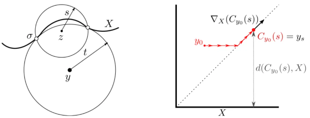
µ. Letσ = ΓX(y)be the set of points in X with minimum distance to y; see Figure 8, left. Suppose the smallest ball enclosing σ has centerz and radius s. Since s ≤ t, we get cX(s) ≤ cX(t) < (1−µ)t and thus t− ky−zk ≤ d(z, X)≤cX(s)<(1−µ)t. It follows that k∇X(y)k= kz−tyk > µ.
Next lemma can be thought of as a converse of the previous lemma, since it provides an upper bound on hX over the interval [0, R], assuming a lower bound on the critical functionχX over the interval(0, R). It extends a result in [7] which says intuitively that the convex hull of point set σ ⊂X cannot be too far away from a shape X, assuming σ can be enclosed in a ball of small radius t and X has a positive reach.
Figure 8: Notation for the proofs of Lemma 11 on the left and Lemma 12 on the right.
Lemma 12. Consider two real numbersµ∈(0,1]andR≥0. LetX ⊂Rnbe a compact set such thatχX(t)≥µfor allt∈(0, R). Then, for all0≤t≤R, one has:
hX(t) ≤ 1 +µ(1−µ)− q
1−µ(2−µ) Rt2
µ(2−µ) R.
Proof. Given σ ⊂ X with Rad(σ) ≤ R and y0 ∈ Hull(σ), we establish an upper bound on d(y0, X) expressed as a function of Rad(σ).
The first step in the proof is to find a point yT that is “sufficiently” far away from X by following an integral line of the generalized gradient ∇X that originates at y0. LetXc =Rn\X. The author in [32] established that there exists a continuous map ΦX :R+×Xc →Xc such that:
d
dt+ΦX(t, y) = ∇X (ΦX(t, y))
where dtd+ denotes the right derivative. Hence,ΦX is a flow and the integral line t7→ ΦX(t, y0) is a rectifiable curve starting at y0. This curve either has infinite length or ends up at a critical point of the distance function to X.
If for some T > 0 the set ΦX([0, T], y0) contains no critical point then it can be parameterized by a continuous function Cy0 : [0, L] → Rn such that Cy0(0) =y0 and the length ofCy0([0, s])iss; see Figure 8, right. Let us prove that under the assumption of the lemma we can choose T = R−d(y0, X).
For all s < R−d(y0, X), we note that d(ys, X) ≤ d(y0, X) +kys −y0k ≤ d(y0, X) +s < R and thereforeχX(d(ys, X))≥µwhich impliesk∇X(ys)k ≥ µ. It follows that the integral line does not reach any critical point as
long ass < R−d(y0, X)andCy0 can at least be parameterized on the interval [0, R−d(y0, X)]. Hence, we can set T =R−d(y0, X). It has been established in [32, 18] that:
∀s∈[0, L), d
ds+d(Cy0(s), X) =k∇X(Cy0(s))k Integrating over the interval [0, T], we get
d(yT, X)−d(y0, X)
T ≥ µ.
Applying Lemma 1 with x=yT and y =y0 gives d(yT, σ)2 ≤T2+ Rad(σ)2 from which we deduce that
(d(y0, X) +µT)2 ≤ d(yT, X)2 ≤ d(yT, σ)2 ≤ T2+ Rad(σ)2. Plugging T = R−d(y0, X), setting δ = d(yR0,X), ρ = Rad(σ)R and rearranging this inequality gives us
µ(2−µ)δ2−2(1 +µ−µ2)δ+ 1−µ2+ρ2 ≥ 0.
Since δ ≤1 we get δ ≤ 1+µ(1−µ)−
√1−ρ2µ(2−µ)
µ(2−µ) , yielding the result.
The upper bound on hX is an arc of ellipse which tends to an arc of parabola as µ→ 0; see Figure 7, right. Note that since hX(t) ≤ t for all t, this upper bound is only relevant when under the diagonal. For µ = 1, we get hX(t) ≤R−√
R2−t2 as in [7]. Equivalently, the graph of hX is below the circle with radius R and center (0, R).
5.3. Reconstructing shapes with a positive µ-reach
Shapes with a positive µ-reach form a large class of objects, that un- like shapes with a positive reach, may possess sharp concave edges. Pre- cisely, for 0 < µ ≤ 1, authors in [17] define the µ-reach of X as rµ(X) = inf{t >0|χX(t)< µ}. The terminology comes from the fact that r1(X) coincides with the usual reach of X.
Given a shape X whose µ-reach is greater than or equal toR > 0 and a finite point set P such that dH(P, X) ≤ ε, we compute the largest value of the ratio Rε for which the Čech complexC(P, α)or the Rips complexR(P, α) provide a topologically correct reconstruction of X for a suitable value of the parameter α. Computations were realized using a computer algebra system and details are skipped. In Appendix C, we give all the details whenµ= 1, R = 1 and n = +∞.
n
εripsn (1) R
n µ∗n
(a)
(b)
(c)
µ2 5µ2+12
λcech(µ)
λrips2 (µ)
λrips+∞(µ)
µ∗2 µ∗∞
µ
Figure 9: (a) Best ratios Rε we can get for a correct reconstruction of a shape with a positiveµ-reach either with the Čech or Rips complex forn∈ {2,3,4,5,+∞}; comparison with the ratio 5µµ2+122 obtained in [17]. (b) and (c) µ∗n andλripsn (1)as functions ofn.
Reconstruction with the Čech complex. Note that our assumptionrµ(X)≥R is equivalent to χX(t)≥ µfor all t ∈(0, R). It follows that a shape X with rµ(X)≥Rsatisfies the hypothesis of Lemma 12 and therefore has a convexity defects functionhX upper bounded by a function that depends uponRandµ.
Plugging this upper bound in Theorem 9, we obtain that ifα+ 3ε≤R then the Čech complex C(P, α) is homotopy equivalent to Xη for all 0 < η < R whenever the following inequality holds for all t ∈[α+ε, α+ 3ε]:
1 +µ(1−µ)− q
1−µ(2−µ) Rt2
µ(2−µ) R < t−3ε.
Eliminating the square root, we can replace the above inequality byHµ,ε(t)<
0whereHµ,ε(t)is a polynomial of degree 2 int. It follows that the above con- dition holds whenever the absolute difference between the two roots t1(ε)≤
t2µ(ε) of Hµ,ε(t) is greater than 2ε. When this happens, the admissible val- ues of α range in the interval Iµ(ε) = [t1µ(ε)−ε, t2µ(ε)−3ε]. The condition t2µ(ε)−t1µ(ε)>2εcan be rewritten as the positivity of a polynomial of degree 2 in ε with two roots, one positive and one negative. Thus, the condition holds whenever ε is smaller than the positive root whose value divided by R is:
λcech(µ) = −3µ+ 3µ2−3 +p
−8µ2+ 4µ3 + 18µ+ 2µ4+ 9 +µ6−4µ5
−7µ2+ 22µ+µ4−4µ3+ 1 . We thus get the following reconstruction theorem:
Theorem 13. Consider a finite set of points P and a compact subset X whose µ-reach R is positive. If
dH(P, X) ≤ ε < λcech(µ)R
thenC(P, α)is homotopy equivalent toXη for allη∈(0, R)and all α∈Iµ(ε).
Interestingly,λcech(µ)does not depend on the ambient dimensionn. Plot- tingλcech(µ)as a function ofµ(see Figure 9(a)), we observe that it is positive for all µ∈(0,1]and improves on the upper bound 5µ2µ+122 established in [17].
Still, for µ= 1, we get λcech(1) = −3+13√22 ≈0.13which is not as good as the value 3−√
8≈0.17obtained in [34].
Reconstruction with the Rips complex. Combining Theorem 10 with β = α and Lemma 12, we get that if ϑnα+ε≤R then the Rips complex R(P, α) is homotopy equivalent to Xη for all 0< η < R whenever
1 +µ(1−µ)− q
1−µ(2−µ) ϑnRα+ε2
µ(2−µ) R < 2α−ϑnα−2ε.
As before, we can eliminate the square root, replacing the above inequality by Hµ(ε, α)<0where Hµ(ε, α)is a polynomial of degre 2 in ε and α. Since we are looking for the greatest value ofεfor whichHµ(ε, α)<0, we may assume that ∂Hµ∂α(ε,α) = 0. Plugging the value ofα for which ∂Hµ∂α(ε,α) = 0 inHµ(ε, α), we get a polynomial of degree 2 in ε whose greatest root εripsn (µ) gives the supremum ofεfor which the above inequality holds. Settingλripsn (µ) = εripsnR(µ) and letting αripsn (µ) be the value of α for which Hµ(εripsn (µ), α) = 0, we get the following reconstruction theorem:


![Figure 9: (a) Best ratios R ε we can get for a correct reconstruction of a shape with a positive µ-reach either with the Čech or Rips complex for n ∈ { 2, 3, 4, 5, + ∞} ; comparison with the ratio 5µ µ2 +122 obtained in [17]](https://thumb-eu.123doks.com/thumbv2/1bibliocom/464361.69875/25.918.166.744.182.587/figure-ratios-correct-reconstruction-positive-complex-comparison-obtained.webp)