The purpose of this task is to develop and compare a set of algorithms used to randomly generate a procedural maze. The goal is to study the set of algorithms that generate perfect mazes and the set of algorithms that generate braids. The proposed algorithm is implemented using 4 different techniques, each of which tries to improve the speed and final form of the algorithm.
The above mentioned algorithms are implemented using python 2.7 with Pygame plugin which is used to implement the maze visualization and its solution. I would like to thank my supervisor, Professor Panagiotis Stamatopoulos, for his help with this thesis. His help and advice were influential and important in the creation of the thesis.
The current thesis was developed within the bachelor's program at the Department of Informatics at the University of Athens. The aim was to develop a set of algorithms capable of generating random mazes of both perfect and interlaced types and visualizing these mazes.
INTRODUCTION
In case the elimination process should create an illegal maze, the algorithm would go back to the previous square that was eliminated and try to find another way to eliminate it. Contrary to the goal of its creation, this algorithm is even slower than the Generate and Test algorithm until the random restart method is used. Using the random restart method, the former algorithm generates mazes quickly, almost as fast as the distribution algorithm, even as the size increases.
However, we must first define what a maze is and its characteristics in order to understand how algorithms use these characteristics to create these mazes (see Chapter 2).
BACKGROUND AND RELATED WORK
Mazes .1 Definition.1Definition
- Dimension
- Hyperdimension
- Topology
- Tessellation
- Routing
Theta Mazes are composed of concentric circles of passages, where the start or end point is in the middle, and the others on the outer edge. A crack maze is an amorphous maze without any consistent tessellation, but instead has walls or passages at random angles. A nested self-levelling maze is a maze with other mazes tessellated within each cell, where the process can be repeated multiple times.
An infinite recursive fractal maze is a true fractal, where the maze contains copies of itself, and is in fact an infinitely large maze. Based on the above definition, we could further classify the maze structure based on the properties of the paths that make up the maze. This type of maze contains only one path from the entrance to the exit, so there are no loops or dead ends in the maze (see Figure 2.6).
A unicursal maze poses no challenge to a player as the player only has to follow the path and he/she is taken directly to the exit of the maze. In contrast, a multicourse maze requires the player to choose which path to follow and therefore requires the player to solve the maze in order to escape.

Maze generation algorithms
Maze solving algorithms
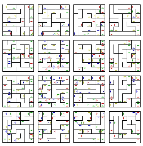
Similarly, a braided maze is an undirected graph containing loops with all edges having a cost of 1, which is the reason why single-cost search[4] can perform the full braided maze search (Chapter 5), while depth-first search in this case does not guarantee the discovery of the shortest path. a) Multiple object maze with dead ends (b) Multiple object maze with loops.

PERFECT MAZE
Recursive Backtracker Algorithm
- Recursive implementation
- Iterative implementation
Second, it can be implemented using an iterative implementation with the help of a stack data structure. A simple way to implement backtracking in an algorithm is with the use of recursion, and this is the first implementation described in this thesis. The reason backtracking is easy to implement using recursion is that there is no need to keep track of which cell we will need to backtrack to, it is already stored on the Python stack.
Each time we need to move to the next cell, we execute a new function that stores all the data needed to execute the part of the algorithm that concerns the new cell. Additionally, when we end the procedure regarding that cell, the return call returns the execution of the program to the previous cell, i.e. generating a function stack for each cell is resource draining, and as the number of cells becomes large, the number of function stacks increases.
To solve this problem, we implement an iterative implementation of the same algorithm using a stack data structure. Instead of relying on the stack to keep track of the cell we need to backtrack to, we keep track of that information inside the stack. Additionally, every time we process a new cell, all of its neighbors are pushed onto the stack.
Kruskal’s Algorithm
Wilson’s Algorithm
BRAID MAZE
- Braid maze generation with probability distribution
- Braid Algorithm Generate and Test
- Pre-Eliminate Squares
- Random restarts algorithm
That is the concept of the first algorithm that we used to generate braided mazes. Next, the algorithm iterates on each cell and randomly assigns a value to that cell based on the probabilities used. In the example given in the previous section, this algorithm is used with the probability that a cell will contain a value of 2, which is 0.7 (see Algorithm 6).
If this test succeeds for every cell in the maze (minus the last row and column, since the evaluation is done indirectly by evaluating all the other cells), then the maze is presented as a result. Although the method of the generation and testing algorithm (Algorithm 4.4) provides a solution in terms of eliminating the squares in the maze, this method is very inefficient and only generates mazes of relatively small sizes. Therefore, while the generate and test technique provides an example of the type of algorithm we want to generate, it does not solve the problem.
For that reason, another algorithm was devised with the primary goal of minimizing the number of squares created while building the maze and ultimately trying to eliminate the squares that were created. First, the algorithm calculates all squares found in the maze, and since the maze is initially empty 4.2, the calculation is made by using the definition of the square and calculating all possible groups of cells that meet the definition. As the amount of these squares is calculated, the algorithm chooses a random square and then a pair at random and erects a wall between these cells.
In the event that this happens, the algorithm goes back to the previous square that eliminated and tries another pair until a valid solution for all squares is constructed. On each square, the algorithm has 4 choices on which wall to lift, and the number of squares is (n−1)∗(m−1) given that the size of the maze is n×m. The pre-eliminate squares algorithm solves the problem faster and for larger mazes than the generate and test algorithm, since the algorithm is allowed to fix the existing squares, instead of waiting for them to randomly disappear from the maze.
However, one problem that arises with the pre-elimination square algorithm is that there are cases where the algorithm makes a choice close to the root of the backtracking tree, leading to an unresolved decision. The idea is that since the first choices are determined randomly, stopping execution, dropping the maze and generating a new maze is cheaper than waiting for a wrong choice to be fixed close to the root of the regressing tree . The algorithm is given a time interval that gradually increases, to try to correct the wrong choices made.
By giving the algorithm this time interval, we ensure that the errors which are deep in the branches of the tree are fixed and at the same time the execution time is not wasted on errors. To summarize, we first define a start time interval t and a number of attempts n, then the pre-elimination algorithm starts running while the execution time is measured.
SOLVER
Class Solver
Class BFSSolver
BENCHMARKS
Analyzing the benchmarks, we notice that Wilson's algorithm [algorithm 4] is statistically the second most efficient algorithm among the four presented algorithms in terms of generating a complete maze (see Figure 6.1d). Occasionally, however, the Wilson algorithm is worse than the recursive Iterative Backtracker algorithm [algorithm 2]. This is expected due to the fact that eliminating squares on the maze reduces the number of walls that the rest of the process has to create, and at small sizes this affects a large percentage of the maze, while as size increases the percentage of the maze filled by the elimination process becomes smaller , and the elimination itself becomes more time-consuming than the rest of the algorithm. We also observe the inefficiency of the Generate and Test algorithm [algorithm 8] and the inefficiency and problematic behavior of the Eliminate Square algorithm [algorithm 9].
We see the effects when in Graph 6.4 the algorithm jumps from 48 seconds to 352 seconds, while only at n = 8 in both cases, making the algorithm even worse than the Generate and Test algorithm. The effect of adding the method of random restarts to the algorithm has obvious results, which confirm the fact that in the search space of the created mazes there is a high probability of finding a solution, which makes restarting the algorithm faster than trying to fix all the squares of the problematic maze. One last conclusion regarding the nature of the problem we are trying to solve is shown in graph 6.7.
By analyzing this graph, we could conclude that creating a perfect maze is less time-complex than creating a woven maze.

CONCLUSIONS AND FUTURE WORK