The "Minimum Spanning Tree" graph theoretic technique addresses some of these problems since an MST depends on the correlation functions of all ranks. The minimum spanning tree technique is used by many scientific disciplines for research or as part of technological solutions.
Thesis statement
Objectives
Contributions
Outline
- A brief history
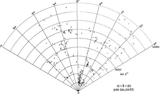
- Large–scale structure of the universe
- Redshift space and distance measures
- Numerical Cosmology
The time evolution of the metric introduces H(z), the Hubble parameter as a function of redshift. Due to the lack of a theory of everything (Laughlin & Pines, 2000), the parameters involved in the evolution of the universe cannot be predicted.
Graph theory
Historical overview
Definitions & examples
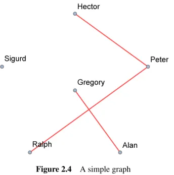
For example, the handshake of the members of the social network in Figure 2.4 could be represented by the graph in Figure 2.7. Note that the spanning tree need not be a subgraph of the graph it spans, as it may contain edges not found in the latter.
Computational Graph Theory and Geometry
- Kruskal’s algorithm
- Prim’s algorithm
- Comparison of the MST algorithms
- Delaunay Triangulation
- Definition
- Estimation
- Other measures
- Computational issues
Kruskal's algorithm (Kruskal,1956) starts with a forest containing all vertices of the input graph, but no edges. Consequently, the time complexity is ElogE and due to the fact that the number of edges cannot exceed 12V (V −1).
Use of MSTs in Cosmology
Delaunay Triangulation and MST
DEUSS
In § 2.3 we analyzed the computational complexity of Kruskal and Prim's algorithms and discussed the optimization possibilities offered by Delaunay triangulation. In the limited time frame of programming, debugging and applying Morava-Pack, the options for algorithms and data structure were inevitably limited.
The logic behind the library
- Programming paradigm
- Representation of graphs, trees and forests
- Input / Output
- Conventions
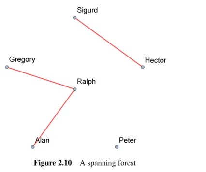
The resulting MST or MSF necessarily contains all the vertices of the original graph and a subset of the edges. MST represents a Minimum Spanning Tree, independent of the original graph, that contains all information: vertices and edges.
Implementation of Kruskal’s algorithm
Pseudocode of our implementation
The size of KFis mentioned in the sense that the current size of a vector is also the index of a newly added element. Output: IndexForestF, so Fi is the list of edge indices (inE2) for the tenth tree in the minimum-spanning forest. Input:EdgesEwhere eKF indices refer to Input:Edges_includedfrom Kruskal algorithm Output:Edges in forestE2 ⊆E.
Implementation of Prim’s algorithm
Pseudocode
The pseudocode for our implementation of Prim's algorithm for complete geometric graphs is listed in Algorithm 4x4.
Implementation of operators
- Pruning a tree
- Pruning a MSF
- Separating a MST
- Separating a MSF
Start from the first edges of the old list of edges and proceed: if the endpoints of the i-th edge are both to be kept, add the edge to the new list of edges. Although the indices of the endpoint of each attached edge still refer to the old top list. Create an array holding the degrees of the vertices in the split tree, initialized to 0.
Delaunay Triangulation
Statistics
- Decriptive statistics
- Fast bootstrap method to estimate the SD of median
- Pseudo–random number generation
- Tree curvature / compactness
In the following sections, an application to the standard error of the median is presented. The sample standard deviation of these is an estimate of the standard error of the median of the original population. Find the smaller of the two values, a, by asking Quickselect to return the bN2c–th element.
Cosmological distance calculations
- Numerical integration
- Interpolant
- Interpolation
- Procedures
- Results
- Discussion
Input : a vectorf of N equal samples of a function Output : The integral of the function over the given range. The result :f vector holds the function evaluations that were used for the last integration. The points are about half (n2 + 1) of the evaluated points outside (n) due to the requirements of Simpson's Rule (even number of intervals.) The latter need not be evaluated as they are already calculated by Algorithm 4.14.
Fast Bootstrap Median
Procedures
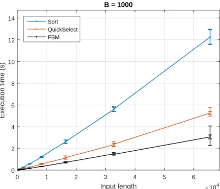
To avoid pathological cases of input and to increase the resolution of timing (for more details, §5.1.1), we measured the time required to process 30 different samples for each input length. By summing the previous values minus one, we can detect the difference due to the even-odd effect, since the input length effect would be negligible for such small lengths. Briefly, we do not provide all the plots for B = 50, as the results were similar to those for B = 1000, except for the errors which were slightly larger.
Results
Error bars were magnified 10-fold and are shown in pairs due to the adjacent input lengths.
Discussion
Distance Calculator
Procedures
The agreement of the DistanceCalcand DEUS-LCDM distance data was verified by producing the motion distance function from the redshift of the halo objects vs.
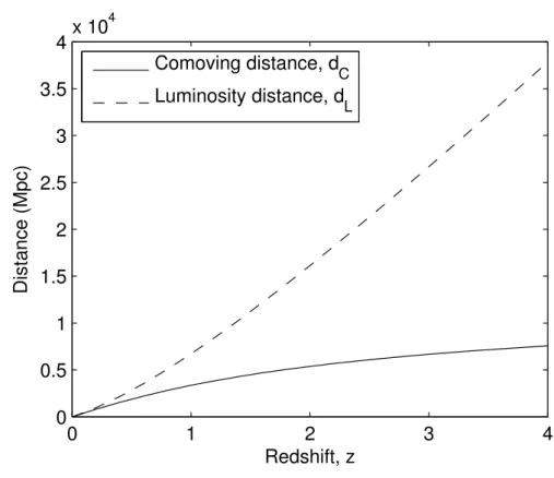
Results
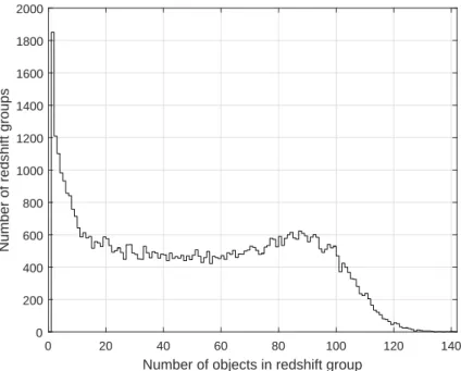
Due to the limited accuracy of the redshift values in the DEUSS data, there were objects with the same redshift but different distances. By sorting the redshifts, finding objects with the same redshift, and averaging their distances, we created a unique and interpolable set of z−dC pairs.
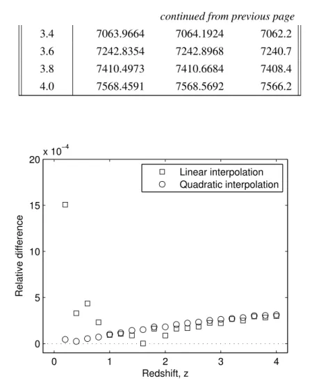
Discussion
The first trend is clearly explained by the fact that the distances compared were 3 to 4 orders of magnitude higher than the accuracy (0.1Mpc) of CosmoCalc (Table 5.2.) The higher the redshift/distance, the higher the error in the relative difference. As we mentioned in the description of the experiment, the DEUSS catalog presented many objects with the same redshift and different distance. When we averaged the distances to create diez –dC interpolation, the «rounding» error in the catalog propagated to the RMSE.
DEUSS MSTs
Procedures
Results
Discussion
In this chapter, we will connect the main points of the thesis and parts of the discussions on numerical experiments (§5.4.3). Due to the limited time frame of the study, the use of cosmological data was not as broad as we would have liked. DistanceCalc was found to be consistent with the CosmoCalc and DEUS catalogs (§ 5.3) in terms of the accuracy level of the latter.
Future work
MoravaPack
The original Prim's algorithm must be available (currently only complete graphs are supported.) Also, choice for the data structure must be added, to suit the user's needs and availability of computing resources.
MoravaGUI
The best programs are written so that computing machines can execute them quickly and that humans can clearly understand them.
Introduction
OpenMP
TetGen
Morava files
Core header file ( mrv_core.h )
Variable types ( mrv_types.h )
In languages with zero-based arrays (such as C, C++, Java, Lisp), a function that searches an array and returns the index of the first occurrence of the key is a legal value. Single argument operators take the index of the coordinate we want to access: 0,1,2forx, y, z respectively. Parentheses operator refers to the index of the ends when the argument is 0 or 1 (from endpoints, respectively) or to the weight when not.
Input / output ( mrv_io.h )
3 Returns false if more than one graph is stored in the file, if count.
Timing ( mrv_time.h)
Built–in metric functions ( mrv_metrics.h )
EuclideanLength returns the Euclidean length (or distance) dE between two points which is equal to the L2 norm (or the Euclidean norm) returned by .
Unweighted graphs ( mrv_dgraph.h )
In the latter case, the function returns whether it succeeded in opening and writing the file. Again, in the latter case, a boolean is returned to confirm success in opening/reading the file.
Weighted graphs ( mrv_wgraph.h )
ClearVertices deletes all vertices but leaves the edges as they are (giving the user more freedom to create other graph organization paradigms). FillWeights(metric) replaces the weight of each edge with the result of applying the metric function to the endpoints.
Finding MSTs / MSFs ( mrv_msffind.h )
CompleteKruskal(metric) clears pre-existing edges, adds all pairs with the weight calculated using the thematic function, and finally calls Kruskal to produce the MST/MSF. CompletePrim(metric) deletes preexisting edges and finds the MST of the complete graph (defined by the given vertices.) The MST edges are preserved. KruskalMST(G, f) finds the MST of the complete graph with the vertices of the Gusing CompleteKruskal algorithm.
MST representation ( mrv_mst.h )
Separate(l, b) separates the tree by cutting edges heavier/longer than l.b is a boolean argument that sets whether it is an absolute length or a parameter multiplied by the mean length of the edges.
MSF representation ( mrv_msf.h )
This allows the user to load/save multiple MSTs in the same file by calling these methods. CombineTrees returns the weighted graph object (see §A.9) with the vertices and edges of all the trees in the forest. If an absolute (b=false) length is given, the separation operator is applied to all trees in the forest.
Delaunay triangulation ( mrv_dt.h )
Random numbers ( mrv_rand.h)
With less than 3 arguments, returns one number in the ranges .. 0.1)(standard uniform distribution) if there is no argument. The following code creates 1000 random numbers from the normal distribution with mean value 2.3 and standard deviation 0.01 and prints one chosen at random. This example also shows why we implemented a single-argument version of Rand_uInt that returns values less than the argument (zero-based arrays/vectors in C++).
General algorithms ( mrv_algo.h )
For example, it can be used for Edges structure since we accommodated the comparison operators in its definition.
Statistics ( mrv_stats.h )
If the sample mean is known, precomputed, etc., it can be passed as the second argument to avoid recalculation. Median calculates the median of the elements of a real vector using the faster method provided in MoravaPack. The second argument (if not given, false is implied) defines sorts the real vector using std::sortof C++STL and returns the median.
Histograms ( mrv_histogram.h )
Therefore, if the vector is not sorted, a partial rearrangement of the elements will occur. LowerBound(i), Midpoint(i), UpperBound(i) return the lower, middle and higher values in the range of the ith bin. RelativeFrequencies,ProbabilityDensities return vectors containing the relative frequencies and probability density estimates of the bins, respectively.
Cosmological distance calculator ( csm_dist.h )
ΛCDM cosmology by setting the hubble parameter and the cosmological density parameter ΩΛ with the assumption that Ωm = 1−ΩΛandΩr = 0 = Ωk. PrintSummary reports the cosmological parameters, the valid range for interpolation, and the number of points used for standard output (usually the screen).
Haloes catalog manipulation ( csm_halo.h)
Clarify the number of halo objects currently in the catalog. COSMOLOGY-ORIENTED CODE Subset(field, oper, key) takes the subset of the halo catalog that meets a comparison criterion: propertyfieldshould be<,=, >,≤or≥to the value key. PROCESS: Create MSTs, DTs, or MSF from the input, or apply operators to created objects.
Notes
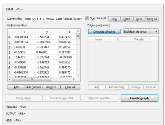
INPUT tab
Check if Complete” informs us whether the graph is complete by confirming that the edge list consists of the expected pairs V(V2−1). Apparently, the speed is achieved by reducing the probability of rejections or equivalently the volume of the cube. The optimal way would be to place any shape so that the major axis of the ellipsoid is parallel to the diagonal of the cube.
PROCESS tab
MORAVAGUI APPLICATION words, we can repeatedly take random points from a cube containing the ellipsoid by treating their coordinates as random variations of uniform distribution, rejecting those outside the ellipsoid. A simple but not optimal way to do this is to fit the ellipsoid into a cube with its faces parallel to the coordinate system axes and sides equal to twice the maximum axis of the ellipsoid.
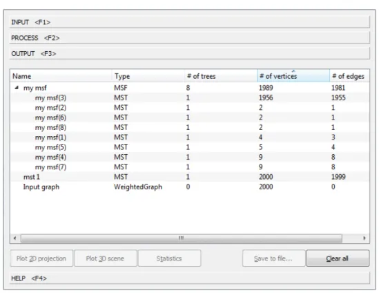
OUTPUT tab
- Greedy MST
- Kruskal’s algorithm
- Prim’s algorithm
- Kruskal’s algorithm
- KF2F algorithm
- MaintainKF algorithm
- CompletePrim algorithm
- Kahan’s compensated summation
- Åke Björck’s modified two–pass algorithm
- Quickselect algorithm
- Median with sort
- Median with QuickSelect
- Fast Bootstrap for Median’s SE
- Discrete uniform rejection method
- Marsaglia Polar Method
- Simpson’s Rule
- Simpson’s Rule with Convergence Check
- Make Interpolation
- Quadratic Interpolation
- Time complexity of Prim’s algorithm
- Computational complexities of MST algorithms
- Properties of DEUSS cosmological models
- Selected MST algorithms for MoravaPack
- Median examples
- Average execution times of MST algorithms
- Cosmic distance calculations
- The DEUSS subcatalogs
- Two sample Kolmogorov–Smirnov tests
- LCDM-1 and RPCDM-1 statistics
- LCDM-3 and RPCDM-3 statistics
- LCDM-5 and RPCDM-5 statistics
- LCDM-1-5 and RPCDM-1-5 statistics
- Distribution of galaxies (CfA)
- Distribution of galaxies (2dF)
- Map of local large-scale structures
- Example of a simple graph
- Example of a directed graph
- Example of a weighted graph
- Example of a complete graph
- Example of a spanning tree
- Example of a minimum spanning tree
- Example of a spanning forest
- Example of pruning and separation operations
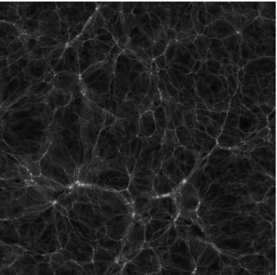
- Black and white slice from a DEUSS simulation
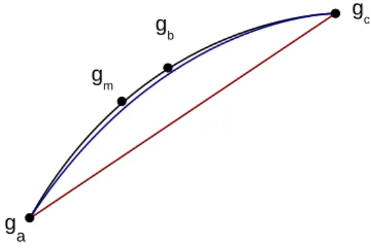
- Detecting a branch
- Linear vs. Quadratic interpolation
- Average execution times of MST algorithms (log–log)
- Average time complexity of Kruskal
- Avarage time complexity of DT + Kruskal
- Avarage time complexity of Prim
- Bootstrap median algorithms comparison (semilog)
- Bootstrap median algorithms comparison (log–log)
- Bootstrap median algorithms speedup (1000 resamples)
- Bootstrap median algorithms speedup (50 resamples)
- DistanceCalc output
- Comparison of cosmic distances
- DEUSS distance verification
- Histogram of redshift groups
- Histogram of redshift groups’ standard deviations
- The MSTs of LCDM-3 and RPCDM-3 catalogs
- LCDM-1 and RPCDM-1 edge length distributions
- LCDM-3 and RPCDM-3 edge length distributions
- LCDM-5 and RPCDM-5 edge length distributions
- LCDM-1-5 and RPCDM-1-5 edge length distributions
The scene is projected on a plane perpendicular to the line joining the observer (behind the screen) and the center of gravity of the points. By pressing «Statistics», the user is prompted for the number of bootstrap samples to be taken to estimate the standard error of the descriptive statistics (see §4.7.2.) After all calculation, a report like the one in Figure C.7 is displayed. Parallel Computation of Median and Order Statistics on GPUs with Applications to Robust Regression.
MoravaGUI’s INPUT tab
Dialog for adding random points
MoravaGUI’s PROCESS tab
MoravaGUI’s OUTPUT tab
MoravaGUI’s 2D plots
MoravaGUI’s 3D plots
MoravaGUI’s statistics report