The first challenge was to study and become familiar with the various concepts in the theory of Quantitative Information Flow (QIF). Within Quantitative Information Flow (QIF) we work in the same context, but we are primarily inter. We can also model different adversaries who might want to leak parts of the information, but not all.
Secrets And Vulnerability
- Probability distribution of X
- Bayes vulnerability
- Guessing entropy
- Shannon entropy
- So how vulnerable is EvilEye Henry’s secret?
The guess entropy is the average number of locations we would have to search to find the true value of X. If the person seeking to discover the secret tries all possible values of Xin in descending order of probability, then the guess entropy is appropriate measure of vulnerability for this case. And if they can ask questions of the form "Does x belong to S?", then Shannon Entropy is the right solution.
Defining g
Calculating gvulnerability
Setting a threshold
And in the one case where the profit is positive, it's just not worth it. This means that if the average profit of an action is lower than the threshold, we never choose that action. Now see what happens if we calculate the average profit for each action and then choose the action with the highest profit.
Channels and Posterior Vulnerability
- Channel matrix
- Prior distribution
- Joint Matrix
- Posterior Distributions
- Finally solving the problem
First, we will answer question number 2, which asks Is the warden's answer useful to Alice. Now, using matrix P, we know that if the guard says Bob's name (P's second column), then Alice has a p(X =A|Y =B) = 13 probability of survival. By the same reasoning, we see that if the warden says Charlie's name (P's third column), then Alice has a p(X =A|Y =C) = 13 probability of survival.
Note that the director never says Alice's name (W never outputs A) and this can be seen by verifying that p(A) = 0. So if the director says Bob's name, you know that your best guess is Charlie and that you have a probability of success 23. Using the same reasoning, we can see that if the director says Charlie's name (the third column of P), your best guess would be Bob, because he has the highest probability in that specific column.
So when the director says Charlie's name, you know your best bet is Bob and you have a chance of success. 23. Before the warden's answer, our best guess as to who the pardoned prisoner is would be, well, anyone, since they have the same chance of being forgiven. But after we receive the director's answer (W's output), we see that we can make a guess with a probability of success of 23.
So, to answer the question, given the warden's answer, the probability of correctly guessing the pardoned prisoner is 23.
Channels and Posterior Vulnerability (part 2)
What if the warden uses a biased coin to answer the question?
So here the keeper's answer is somewhat useful to Alice, meaning that it updates her knowledge about the probability that she will survive in some cases.
Which means that whatever p the manager uses to determine his answer, our best guess will always succeed with probability 23. You could say that all W defined in this way are equally vulnerable to someone trying to guess pardoned prisoner in one attempt. For more insight into why this is happening, take a look at the following piece of code.
For each pfrom0to1 it prints thepparameter itself, then the distributionpY(y) fory=BorC(remember that Alice's name never appears, which means pY(A) = 0, so y = A is omitted) and then the array of the later distributions. Notice how the maximum elements of each column remain at the same positions as p increases. It means that when observing a specific output, our best guess always remains the same, regardless of the distribution of X.
Channels and Posterior Vulnerability (part 3)
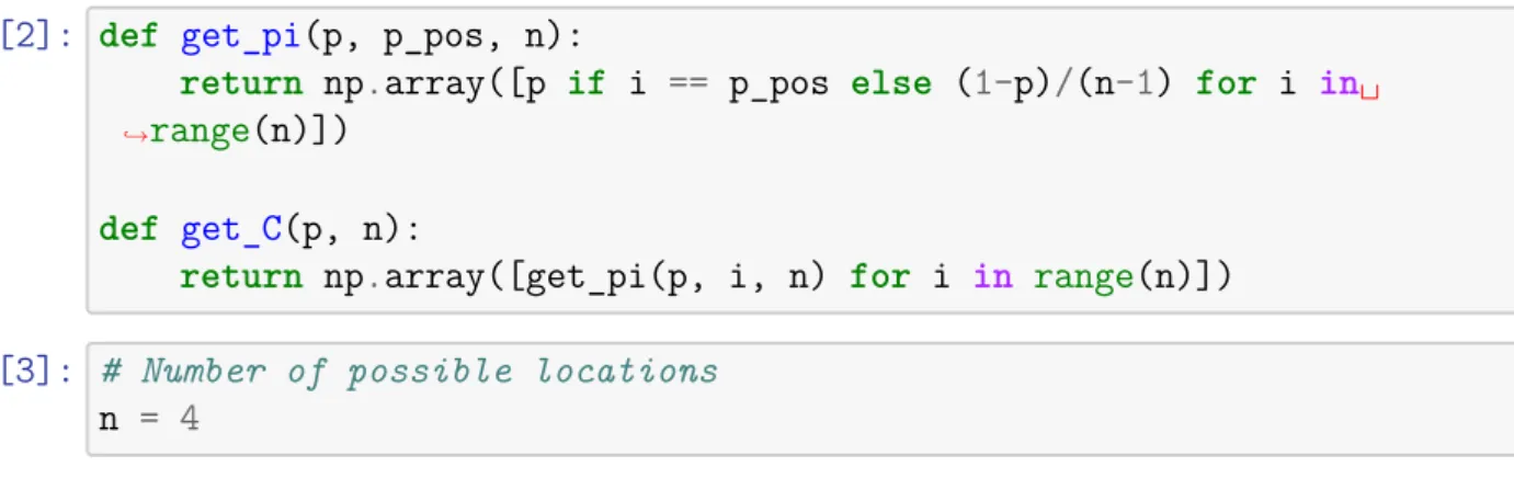
- What if the pardoned prisoner is not uniformly chosen at random?
- Prior vunlerability
- Posterior vunlerability
- Multiplicative leakage
- Generalizing over any prior distribution
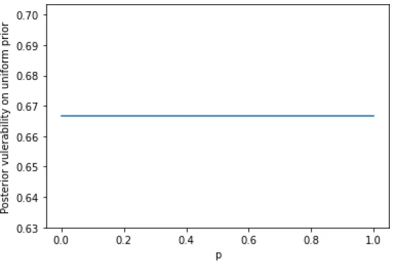
The x-axis corresponds to the pparameter of get_distribution(p) and the y-axis to the vulnerability of the distribution produced by get_distribution(p). The code below prints the corresponding distribution for each parameter and highlights the element with the highest probability, which is essentially our best guess for that par. For p = 13, our best guess is A, B, or C, and this gives us the minimum probability of success under all possible values of p.
Xaxis again corresponds to the pparameter ofget_distribution(p) but now yaxis corresponds to the posterior vulnerability of W when based on distri. The following code prints for each p the parameter p itself, then the distribution npY(y) for y = B or C (remember that Alice's name never appears which means pY(A) = 0, so y = A is omitted ) and then the range of posterior distributions. Both the prior and the posterior vulnerability are equal to 109, which agrees with the fact that the multiplier effect is 1.
It is also interesting to note that L×(π, W) has an inflection point atp= 13, the same point where the previous vulnerability turns. It also has another one at p = 12, the same point where the posterior vulnerability turns. For any channel C, the maximal multiplicative Bayes leakage over all priors is always realized on a uniform priorθ.
So according to this theorem, we can be sure that there is no prior vulnerability that makes the posterior vulnerability of our channel greater than twice the prior vulnerability.

Refinement
- Producing the actual location with probability p = 0.7
- Producing the actual location with probability p = 0.6
- Comparing C 1 and C 2
- Different p for some rows
Here, the posterior vulnerability corresponds to the probability of guessing the actual location by observing the C1 output of the location. Note that its posterior vulnerability is again equal to thepparam, which is the probability that the actual location appears on the output. Perhaps a specific adversary has some other prior knowledge of what our true location might be before observing the chan.
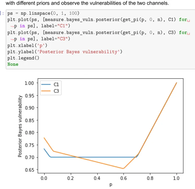
But if we want to be sure that this happens for every possible prior distribution (or even for every possible gain function), then we need to check for accuracy. This means that there is a channel R that receives each output of C1 and processes it further, pro. Here we see that for some prereleases, C1 has the least vulnerability of the two, and for other prereleases, C3 has the least vulnerability.
This means that an adversary with a different knowledge of the prior distribution might prefer one channel over the other. However, as seen in the plot above, one channel may be more vulnerable than the other to others in the past. Absence of refinement also means that even under the same prior distribution π there can be one opponent who prefers C3 and another who prefers C1.
Notice how opponentkg1 prefers C3 because it has the highest vulnerability of the two, while forg2's best choice is C1.

CASE STUDIES 50
Computing the vulnerability of W
If we take a look at the hyperdistribution of W, we see that each outcome occurs with the same probability, and by observing it, the possible voting combinations also occurred with the same probability.
Computing the vulnerability of C
Comparing the two channels
And it would not be a surprise to anyone if they have observed that C is a post-processing of W or in other words, C is a refinement of W. It can also be realized more intuitively if you think about the process of announcing the winner of the election. First, the votes for each candidate are tallied (which is what W does), then they are compared to see who has the most, and finally the winner's name is announced.
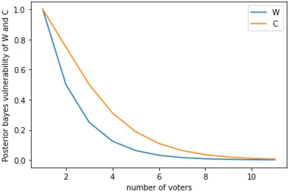
Thus, the process of comparing the votes for each candidate and deciding who has the most votes is the post-processing of W. This stems from the fact that as the number of voters increases, the number of possible outcomes also increases, ultimately resulting in a more detailed distribution of Y. So far we have been using Bayesian vulnerability, which is equivalent to an adversary trying to correctly guess the entire vote combination. occurred.
Different Adversarial Models
- Adversary 1
- Adversary 2
For any announcement of scores for an election whose voting pattern is z, most voters voted for the candidate with the majority, and so the ad. Since the optimal guessing strategies are therefore the same for both W and C, the leakage with respect tog1 must also be the same. Another adversary can benefit if they can find a voter/candidate pair such that the voter did not vote for that candidate.
Note that G0 is the complement of G1, meaning it is the result of interchanging the 1s with the 0s and vice versa. But as it turns out, for 3 candidates or more, this type of adversary has more to gain in elections where they announce the votes for each candidate (ie, channel matrixC). Recall that the posterior vulnerability under g0 gives us the probability that an adversary correctly guesses what a voter did not vote for.
When the tallies are announced, an opponent can increase their profits by guessing that the candidate who received the fewest votes is most likely not someone the voter chose.

Differential Privacy
- An example scenario
- Assesing information leakage through QIF
- Assesing information leakage through Differential Privacy
- Comparing the two approaches
WhatHdoes is basically adding noise to the true answer and it does this using a (truncated) geometric mechanism with a parameter of a = 13. So we pick the maximum probability for each column and then weight each one by its outer probability ie. We keep the largest ϵ from each column of C so that the above inequality holds for all columns.
We check that this is indeed the worst case of ϵ by observing the values of ϵ for each column of C. Another way to think about this is that we measure different privacy for each column of C. QIFvulnerablity measures the probability that an adversary will correctly guess the secret x (i.e. the entire database in our case) by observing the channel output.
Going a little further, we see that QIF vulnerability is sensitive to the prior distribution of X, while differential privacy is not. Another difference between the two is that QIF vulnerability is defined as the result of the average contribution of all the columns to the vulnerability, while differential privacy represents the worst case (i.e. the maximumϵfor allz). So there may be a column with a very high ϵ value that does not contribute much to the mean (typically because the corresponding output has a very low probability of occurring).
In that case, the QIF vulnerability could be very small, while the differential privacy would still have a very large value.
Posterior vulnerability on uniform prior
Prior vulnerability with original W
Posterior vulnerability with original W
Multiplicative leakage with original W
Posterior Bayes Vulnerability
Posterior Bayes Vulnerability
Posterior Bayes Vulnerability of W and C
Multiplicative Bayes Leakage of W and C
Multiplicative Leakage of W
Multiplicative Leakage of C
One thing to note is that the true answer from has the highest probability within its row. The following image graphically represents the entire environment (leave aside the concepts of leakage, age and usefulness for the time being). This is also evident from the fact that the get_worst_epsilon function does not use an API parameter.
Multiplicative Leakages of W and C
Leakage and utility for oblivious mechanisms
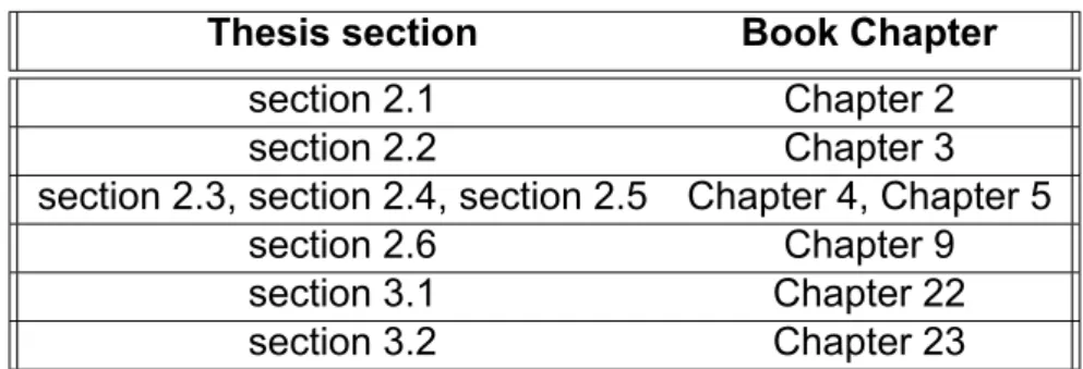
Thesis sections and book chapters matching
C 1 matrix
C 2 matrix
C 3 matrix
W matrix
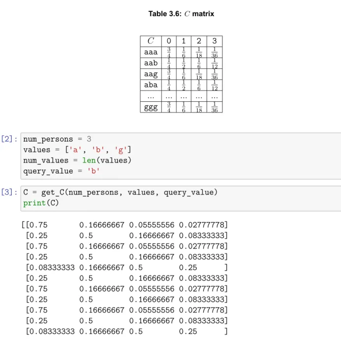
C matrix
H matrix
C matrix