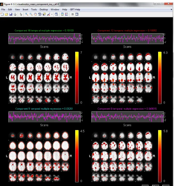
65 Figure 4-10 Selected projections of 4 components after being temporally sorted using multiple regression on all data over all time courses. 66 Figure 4-11 Selected projections of 4 components after being sorted temporally using multiple regression on all data over all time courses.
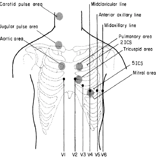
Electrocardiogram (ECG)
The PR interval is measured from the beginning of the P wave to the beginning of the QRS complex. The QT interval is measured from the beginning of the QRS complex to the end of the T wave.
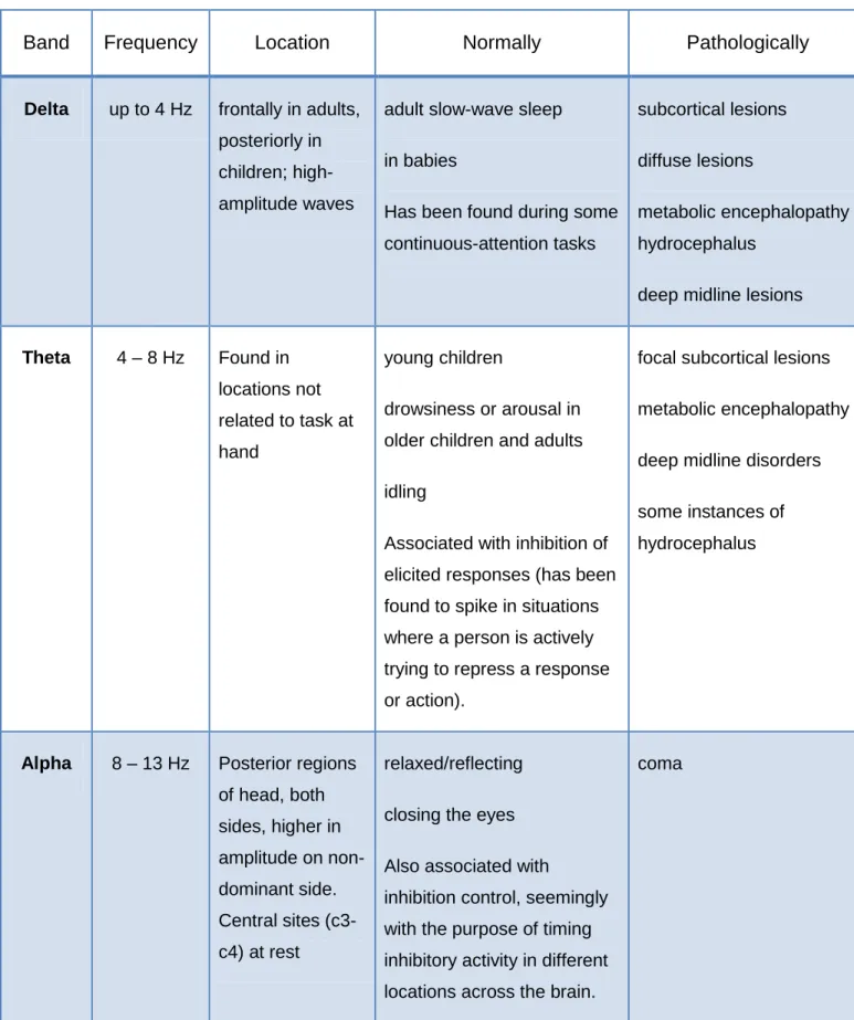
Electroencephalogram (EEG)
Recording Methods
In addition, one or two reference electrodes (often placed on the earlobes) and a ground electrode (often placed on the nose to provide reference voltages to amplifiers) are required. When such bipolar electrodes are placed close together (say 1 or 2 centimeters), potential differences are estimates of tangential electric fields (or current densities) in the scalp between the electrodes.
International 10–20 system
Derivatives of the EEG technique include evoked potentials (EP), which average the EEG activity time-locked to the presentation of some stimulus (visual, somatosensory, or auditory). Two anatomical landmarks are used for the essential positioning of the EEG electrodes: first, the nasion, the distinctly depressed area between the eyes, just above the bridge of the nose; second, the inion, the lowest point of the skull from the back of the head and normally indicated by a prominent bump ( Towle et al., 1993 ).
Waves and Artifacts
Glossokinetic artefacts are caused by the potential difference between the floor and the tip of the tongue. Poor grounding of the EEG electrodes can cause significant 50 or 60 Hz artifact, depending on the frequency of the local electrical system.
Magnetic Resonance Imaging
Basic MRI scans
- T1-weighted MRI
- T2-weighted MRI
- T*2-weighted MRI
- Spin density weighted MRI
T1-weighted scans refer to a set of standard scans that show differences in the spin-lattice (or T1) relaxation time of different tissues in the body. Gradient-echo-based T1-weighted sequences can be acquired very quickly due to their ability to use short inter-pulse repetition (TR) times.
Specialized MRI scans
- Magnetic resonance angiography
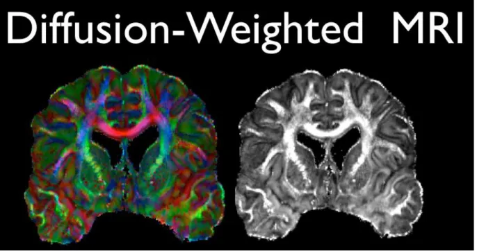
- Diffusion imaging
- Real-time MRI
- Functional MRI
The main application is imaging white matter, where the location, orientation and anisotropy of the tracts can be measured. This vector can be color coded, providing a cartography of the position and direction of the orbits (red for left-right, blue for superior-inferior, and green for anterior-posterior). Fiber tracking algorithms can be used to track a fiber along its entire length (for example, the corticospinal tract, through which motor information passes from the motor cortex to the spinal cord and peripheral nerves).
The localization of tumors in relation to the white matter tracts (infiltration, deflection), was one of the most important initial applications. When an area of the brain is in use, blood flow to that area also increases. Another form is changes in the current or voltage distribution of the brain itself which causes changes in the receiver coil and reduces its sensitivity.
The inverse problem
- Dipole fitting
- Minimum norm based approaches
Because of the underdetermination of the problem, blind source separation methods generally seek to narrow the set of possible solutions in a way that hardly excludes the desired solution. Regardless of the specific system type, blind signal processing includes three main areas, depending on whether we want to extract the input signals or the system parameters: Blind Signal Separation and Extraction, Independent Component Analysis (ICA) and Blind Multichannel Blind Deconvolution and Equalization. In blind source extraction, our goal is to recover the source(s) given the observation signal.
In the case of BSS, the linear system can be instantaneous or convolutive (general MIMO). In blind system identification, our goal is to obtain the system parameters rather than recover the source signals. If the system includes non-trivial convolution, the goal is to extract the filter taps.
The linear BSS problem
If there is more than one source, the problem is called blind source separation (BSS). In the case of blind deconvolution (BD), we want to invert a linear filter, which of course operates on its input via a convolution operator, hence the name "deconvolution" given to this problem. The source separation/extraction problem has an inherent ambiguity in the order and extent of the sources: the original signals cannot be retrieved in their original order or extent unless additional information is available.
If no a priori information is available, the latter is only possible up to arbitrary permutation and scaling. In a specific case where the matrix is square (i.e.) and invertible, and under the assumption of no noise, the problem is equivalent to estimating the unmixing matrix. A detailed description of each technique is beyond the scope of this study and the reader is referred to the works cited.
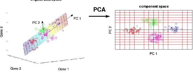
Principal component analysis
The central idea of PCA is to reduce the dimensionality of a data set consisting of a large number of interrelated variables, while preserving as much of the variation present in the data set as possible. This is achieved by transforming into a new set of variables, the principal components (PCs), which are uncorrelated and arranged so that the first few retain most of the variation present in all the original variables. Briefly, PCA is an orthogonal linear transformation that transforms a set of observations of possibly correlated variables into a new coordinate system such that the largest variance of any data projection lies on the first coordinate (called the first principal component), the second largest variance on the second coordinate, and so on ( Jolliffe, 2002).
Left: Using PCA, we can identify the two-dimensional plane that optimally describes the highest variance of the data. If mean subtraction is not performed, the first principal component may roughly correspond to the mean of the data. A mean of zero is needed to find a basis that minimizes the mean square error of fitting the data (Miranda et al, 2008).
Independent Component Analysis
Basic System
- Linear noiseless ICA
- Linear noisy ICA
- Nonlinear ICA
The data is represented by the random vector and the components as the random vector. The components of the observed random vector [ ] are generated as a sum of the independent components. This is done by adaptively computing the vectors and setting up a cost function that either maximizes the non-gaussianity of the computed one.
In some cases, a priori knowledge of the probability distributions of the sources can be used in the cost function. The original sources can be recovered by multiplying the observed signals by the inverse of the mixing matrix, also known as the demixing matrix. With the additional assumption of zero-mean and uncorrelated Gaussian noise, the ICA model takes the form.
Fast ICA
An iterative algorithm finds a direction for the weight vector that maximizes the non-Gaussian projection for the data. The non-Gaussian property maximization method should be extended to estimate multiple independent components. For simulated data, this algorithm performs better in terms of spatial correlation of the estimated sources with the original sources for super-Gaussian sources compared to other sources.
For a smaller number of components, FastICA with Gaussian nonlinearity provides better performance compared to the other two nonlinearities for Gaussian and sub-Gaussian sources. Convergence is cubic (or at least quadratic), under the assumption of the ICA data model. This is in contrast to many algorithms, where an estimate of the probability distribution function must first be available and the nonlinearity must be chosen accordingly.
JADE OPAC
EVD
AMUSE
SIMBEC
Infomax
ERICA
Constrained ICA
SOBI - COMBI
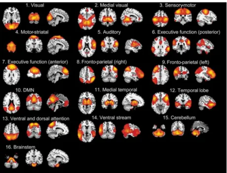
There are three main phases to Group ICA; Data compression, ICA and ridge reconstruction (Calhoun et al., 2001). For applying BSS methods to selected biomedical signals, the GroupICATv3.0a version of the Group ICA Of fMRI Toolbox was used (Calhoun et al., 2003; Calhoun et al., 2004). It is a MATLAB toolbox that implements several algorithms for independent component analysis and blind source separation of group (and individual) fMRI data (GIFT) and EEG data (EEGIFT).
For detailed information on the methods and utilities provided by the Toolbox, the reader is referred to the cited material. This will be followed by a small presentation of the tools, a comparison of the selected BSS methods and their results. FastICA was chosen to perform the single-run and multi-run analysis (ICASSO), which determines component reliability and method stability, and Infomax was chosen for the multi-run analysis.
FastICA
- Single run
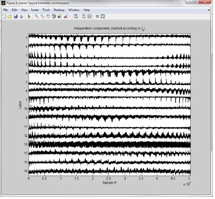
- ICASSO
Only FastICA will be shown in single run to demonstrate the existence of artifacts due to the components not being optimally separated. Due to the nature of the paradigm (appendix), the alternating visual stimuli and the simultaneous motor task can be seen in Figures 4-6. It should be noted that a single-run ICA does not always give good results, and several runs with the selection of the persistent components (refined from artifacts and random components) are recommended.
Another interesting phenomenon is when a component is split in two, as happens in Figure 4-11 on the DMN network. On the composite image (Figure 4-12) of the components, one can see the spatial and temporal overlap that creates the DMN network. Above) the DMN network is divided into 2 components, (bottom right) component looks like attention network.
INFOMAX
34;Low-field magnetic resonance imaging of polarized noble gases obtained with a "DC" superconducting quantum interference device, Applied Physics Letters. Latency-sensitive ICA ensemble independent component analysis (in) of fMRI data in the temporal-frequency domain. A method for group comparison of fMRI data using independent component analysis: application to visual, motor and visuomotor tasks.
Jirsa VK and Haken H (1997) A derivation of a macroscopic field theory of the brain from quasi-microscopic neural dynamics. Efficient variant of the FastICA algorithm for independent component analysis that achieves the Cramér-Rao lower bound. Le Bihan D., Urayama S., Aso T., Hanakawa T., and Fukuyama H., (2006) Direct and rapid detection of neuronal activation in the human brain by diffusion MRI.