In this new method, the free surface calculated by means of the potential solver is corrected via a surface tracking RANS method. Most commercial CFD software uses some sort of surface capture method for calculating the free surface.
Literature Survey
- Total Variation Diminishing Schemes
- Free Surface Calculation Methods
- Methods for Solving the Flow around Ship Appendages
- Methods for Overlapping Grid Blocks
The Surface Tracking methods have been shown to be very accurate in calculating the free surface and are therefore more suitable for drag or propulsion calculations (Papakonstantinou & Tzabiras, 2002, Wilson et al., 2006). These methods try to solve even the more complex problem of the propeller operation (Shen et al., 2015).
The LSMH Method for Solving the Flow around Ships
Another approach to the ship plugging problem is that of nested structured grid blocks. The grid blocks are orthogonal curved in the UV directions thus increasing the accuracy of the method.
Thesis Outline
At the end of this chapter, the proposed method for exchanging flow variables between blocks is detailed. Finally, drag and propulsion calculations were performed for the ship with the rudder, in model and full scale.
The Governing Equations
The Navier-Stokes Equations
Curvilinear Coordinates
Turbulence Modeling
The Reynolds Averaged Navier-Stokes Equations
Rather inconveniently, a total of six new unknown quantities appear on the right-hand side of the RANS equations, called Reynolds stresses. Where the effective viscosity μe is calculated as the sum of the dynamic viscosity μ and the eddy viscosity μt:.
The Two-Equation k-ε Model
The RANS equations together with the continuity equation and the k and ε equations form a system of six equations with six unknown quantities, three velocity components, pressure and turbulent kinetic energy and its dissipation rate.
The Two-Equation k-ω-SST Model
In the wake or the regions far from the fixed boundary, turbulence is only modeled using the k-ε model, i.e. The source of turbulent kinetic energy is calculated through the eddy viscosity and the deformation tensor, in the same way as in the k- ε model:.
The Finite Volume Method
- Introduction
- The Differencing Scheme
- Total Variation Diminishing Schemes
- Boundary Conditions
- Pressure Correction Algorithm
In terms of the Taylor series truncation error, the Upwind Differencing scheme is a zero-order scheme. The Central Differencing scheme is second order in terms of the Taylor series truncation error.

Geometrical Representation of the Hull
- Introduction
- The Conformal Mapping Method
- Interpolation of Sections
- The Conformal Mapping of Doubly Connected Regions
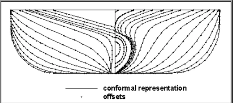
Where P is the number of data points (xP, yP) describing the contour of the section and (xaP,yaP) the corresponding analytical expressions through equation 2.4.2. The corresponding layout of the intermediate station is quite close to the real offsets (figure 2.4.4).
The Numerical Grid
- Introduction
- The Conformal Mapping Method for 2-D Grids
- The Bow Grid Block
- The Grid Block around the Midship and Stern
- The Wake Grid Block
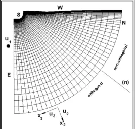
Figure 2.5.4 shows the conformal map of such a section, while Figure 2.5.5 shows the resulting 2-D network. In the case of a ship with a bulbous bow, a C-O grid block is created around the bow and part of the midship.
The Actuator Disk Method
Then thrust is considered equal to the drag and the body forces are calculated for given propeller geometry (tip and hub diameter, sweep circumference), shape of circulation distribution and propeller efficiency. The thrust is set equal to the new value for the resistance, the new body forces are calculated and the flow problem is solved again.
RANS Free Surface Calculations
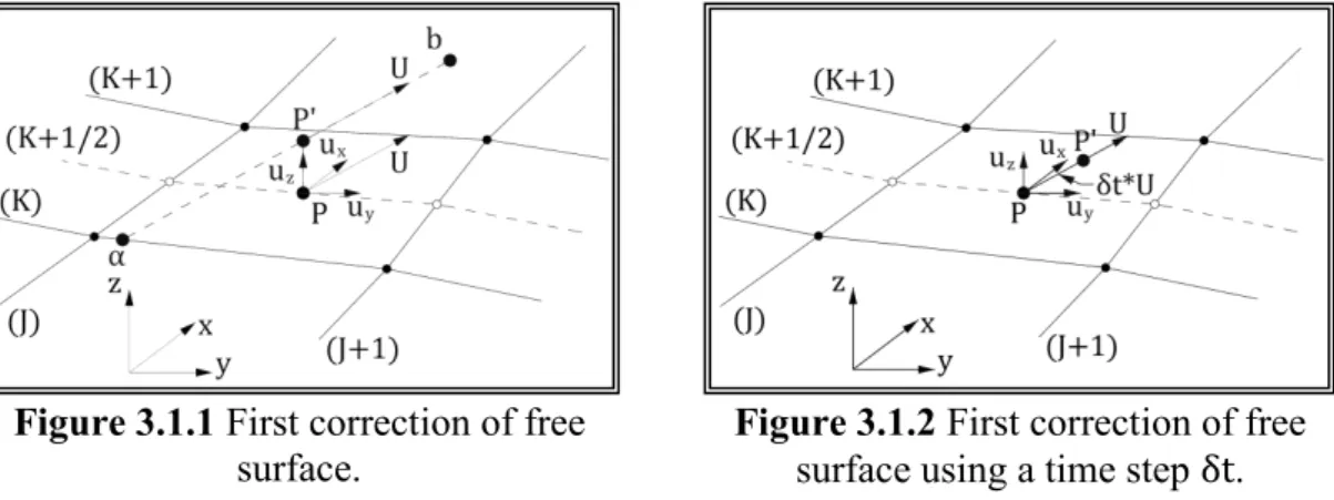
The location of the points P' does not coincide with the cross-sections of the original surface. To be compatible with the convergence of the continuity equation, (ABCD) coincides with the north side of the free surface pressure control volume. The fulfillment of the kinematic boundary condition is tested using the average value of the correction obtained from equation (3.1.1) |δz|�����.
Due to the approximation of the free surface to the quadrilateral panels, this value decreases as the problem converges, but exhibits a limiting behavior.
Potential Flow Free Surface Calculations
- The Potential Flow Problem
- The Hess & Smith Method for Potential Flows
- The Numerical Method of Solution
- The Free Surface Calculation
- Wave Making Resistance, Sinkage and Trim Calculations
The term 2πσ(p) is the contribution to the outward normal velocity at a point p on the source density boundary in the immediate vicinity of p. The integral term represents the contribution of the source density on the remainder of the boundary surface to the outward normal velocity at p. The normal velocity induced at the control point of the ith element by a unit source density at the jth element is.
Flow quantities on the hull and water surfaces are calculated only at element control points.

A Hybrid RANS-Potential Method for Free Surface Calculations
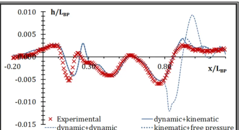
In the figures below, the solid lines correspond to a numerical solution where along the stationary part of the surface the dynamic boundary condition for the transport equations is applied while the kinematic condition is applied during the pressure correction. The dashed lines correspond to a numerical solution where along the fixed part of the surface the kinematic boundary condition for the transport equations is applied and the pressure also satisfies the dynamic condition. Finally, the dotted lines correspond to a numerical solution where along the fixed part of the surface the kinematic boundary condition for the transport equations is applied and the pressure is determined through the Neumann condition normal to the water surface.
When staring with the surface as calculated by the potential rescuer, approximately 100-200 steps are required to correct the free surface around the stern.
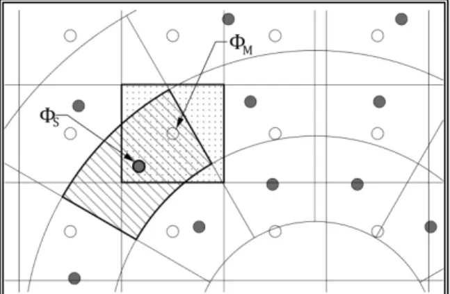
The Overlapping Grid Block Method
That is, for all flow variables bar pressure, the conditions are derived from the solution of the Master grid, while Neumann conditions are applied for the pressure. This procedure is followed for each finite volume on the external boundaries of the slave grid (figure 4.1.3). This time the conditions are not imposed on the boundaries of the Master Block but on internal finite volumes.
Then the main network block is resolved, applying the conditions obtained from the slave in the closed loop and leaving the volumes inside the loop empty, i.e.

The Geometrical Problem, the Appendages of a Ship
Specifically, each part of the shaft between two objects will be modeled as a cylindrical block. If we consider the example of a twin-propeller ship with a shaft supported by one V-beam, then there will be one grid block for the shaft projection, and another for the part of the shaft between the shaft projection and the V-type beam projection, two blocks for two struts, one block for the protrusion of the struts and finally a further cylindrical block for the part of the shaft, for the protrusion of the struts. In the case of a ship with one type I-girder and a further type V-girder, the grid blocks would be those of the previous example, plus one block for the type I-girder strut, one block for the I-girder bulge, and a third cylindrical block for the shaft section between the two girders.
By adopting the above subdivision, most cases of the complex attachments found on ships can be modeled using a small number of grid block types.
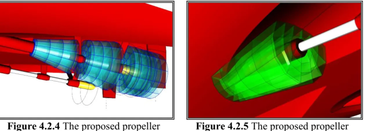
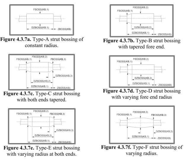
Geometrical Representation of the Appendages
At the forward end of the propeller hub, the diameter may match the diameter of the rear strut riser. The first angle is calculated as the linear interpolation of the angles of the two input sections. The hydrofoil profile on each of the two inlet sections is defined by a number of points.
In the first case, the shape of the handlebar is defined by two parts, one at the tip and one at the bottom.
Generation of a General 2-D Orthogonal Curvilinear Grid
Figures 5.2.5 (a) and (b) show the distribution of the pressure coefficient cp at the solid boundary.
The Propeller Shaft Grid Block Generation
The Propeller Shaft Bossing Grid Block Generation
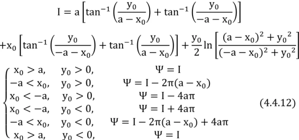
The Struts Bossing Grid Block Generation
The Struts Grid Block Generation
The Rudder Grid Block Generation
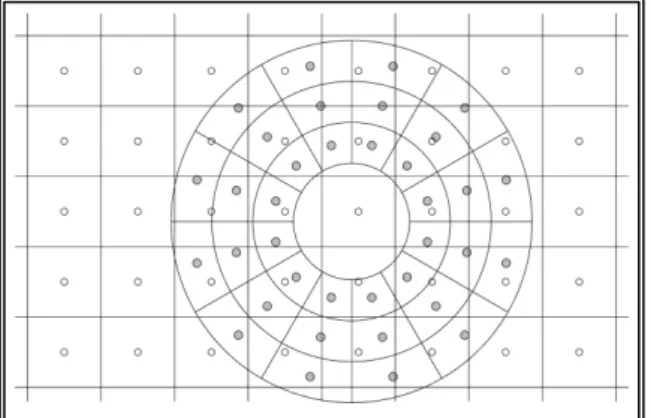
Exchange of Flow Variables between Grid Blocks
Inclusion Test
Finally, the planes of the child 2-D meshes generally do not coincide with the planes of the main 2-D meshes, i.e. with respect to the coordinates of a point p, say the center of the volume of the child grid, a triple shift along the K ,I,J direction of the main grid. Then the intersection c of the segment [ab] and the line normal to [ab] and passing through p is located.
In figure 4.10.3, an application of the above method is shown, for the northern border of the slave network of figure 4.10.1.
Interpolation of Flow Variables
Let's say that PS is located between two sections of the main grid, sections K and K+1. From the inclusion test of the previous paragraph, we obtained the K-way weighting factor WFK. The bi-linear method starts by locating the master volume that contains the center of the slave volume PS.
The centers of pages K, K+1 of four neighboring volumes form a new volume, a total of four new volumes (figure 4.10.5).
Rotation of U, V Velocity Components
The Proposed Solution Procedure
Next, the front ash block is solved (Figure 4.11.3), where the boundary conditions for the inflow (K=1, upstream) boundary come from the solution of the ash forest block. The downstream boundary (K=NK) is treated as an outer boundary with conditions taken from the solution of the truss block and possibly the ash block that follows. Boundary surface definition for transferring the flow variables from the attachment blocks to the ship block.
The Downstream (K=NK) and North (J=NJ) boundaries are treated as external boundaries with conditions taken from the ship block solution.
Introduction, the 200/08 LSMH model
Flow Calculations about the Propeller Shaft
Propeller Shaft Calculations, Forward Section
Specifically, the mass residual is shown as a function of the steps of the pressure correction algorithm. In Figures 5.2.6 to 5.2.8, the current traces are presented on one longitudinal section of the current field. In the same figures, the contours correspond to the in-plane velocity intensity divided by the far-field velocity.
Propeller Shaft Calculations, After Section
The presented method can generate numerical meshes around different ship propeller shaft configurations, considering possible steps in the shaft diameter. The modified RANS solver can now handle the O-type shaft block with the above steps. It is also demonstrated that the solver can produce realistic results in terms of flow characteristics and pressure distribution on the shaft surface.
However, further examination is required to determine the required mesh density and to validate the integrated values produced, such as shaft pull.
Flow Calculations about the Propeller Shaft Bossing
This is mainly the result of the unrealistic boundary conditions (uniform flow) especially on the outflow (downstream, K=NK) boundary. In figures 5.3.14 to 5.3.16 the distribution of the pressure coefficient cp on the solid boundary is presented. In this paragraph it is demonstrated that the solver can produce realistic results in terms of the flow characteristics and the pressure distribution on the thrust surface.
The method also requires validation in terms of the integrated values produced, such as the increase in vessel resistance.
Flow Calculations about a Strut
This is primarily the result of the unrealistic boundary conditions (uniform flow) in connection with the narrow width of the strut block. In figure 5.4.7, the convergence history of the drag coefficient (CD) is presented as a function of the steps of the pressure correction algorithm. In figures 5.4.8 and 5.4.9, the pressure coefficient contours are shown on the two sides of the strut.
This paragraph shows that the solver can produce realistic results in terms of flow characteristics and skin pressure and friction distribution on the strut surface.
Flow Calculations about the Rudder
Figure 5.5.9 presents the convergence history for the drag coefficient (CD) as a function of the steps of the pressure correction algorithm. This paragraph shows that the solver can produce realistic results in terms of flow characteristics and pressure and skin friction distributions on the rudder surface. The method also requires validation in terms of produced integrated values such as steering resistance.
Such an investigation is presented in the case of the "Dyne" tanker, in Chapter 6. FLUID CALCULATIONS OVER THE RUDDER.
Introduction, the “Dyne” Test Case
For self-propelled tests, the model is equipped with a propeller model, set at X/LPP=0.989, measured from the Front Perpendicular.
Free Surface Calculations
- Model Scale Resistance Calculations, Symmetric Flow
- Model Scale, Near Wall Treatment Resistance
- Model Scale Propulsion Calculations, Symmetric Flow
- Model Scale Resistance Calculations, Asymmetric Flow
- Model Scale Propulsion Calculations, Asymmetric Flow
- Full Scale Resistance Calculations
- Full Scale Propulsion Calculations
In addition to the integrated values, flow variables are also presented on four parts of the ship near the stern (figure 6.3.1). In the numerical self-propulsion tests, the propeller is modeled via the actuator disk method (section 2.6) and the propeller characteristics are those of the “Dyne”. In the first set of tests, the problem was considered symmetric and only half of the computational domain was modeled.
In order to evaluate the accuracy of the wall function approach (paragraph 1.4.4) used in the previous test, the same problem was solved using the near wall treatment approach this time.
The Overlapping Block Setup for the Rudder
Overview of the Overlapping Block Setup
Grid Independence Tests for the Rudder Grid Block
Hull and Rudder Calculations
Discussion on the “Dyne” Test Case
Novel Contributions and Relevant Publications
Future Work