Comparison of the decays B→J/ψK, J/ψ → µµ and B→ µµK with the CMS experiment at CERN LHC

The direct decay B± → µ+µ−K± involves a taste-changing neutral current (FCNC), and is therefore forbidden at tree level in the Standard Model. FCNC rare decays of B mesons are particularly interesting, as they probe Lepton flavor universality in the weak interactions.

The Large Hadron Collider

Thus, unfortunately, the total available energy within the parton center of mass is always lower than 13 TeV. The available energy within the parton center of mass determines the possible particles produced, since particles with a mass greater than the available energy are strictly forbidden to be produced.

Figure 1: The CERN accelerator complex [30].

The Compact Muon Solenoid - CMS

Tracking System

The pixel tracker forms the core of the detector and deals with the highest intensity of particles. Much of the technology behind tracker electronics emerged from innovation in collaboration with industry.

Figure 4: Sketch of a typical CMS pixel sensor

The Electromagnetic Calorimeters

The homogeneous nature of the ECAL crystals reduces the stochastic term by minimizing the loss of scintillation photons in the absorber. However, the light yield emitted in the active material is quite low (~50 photons/MeV), and varies with temperature (-2%/low 18oC).

Figure 6: Simulated cascades inside electromagnetic crystals.

The Hadronic Calorimeters

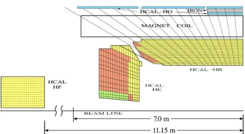
In the trigger path, the trigger primitives received from the electronics on the detector are synchronized by the trigger concentrator cards and sent to the regional calorimeter trigger. The effective HCAL thickness in the range|η|<1.3 is increased by the addition of the outer barrel (HO) scintillators outside the magnetic cryostat.

Figure 8: A quadrant of the CMS hadronic calorimeter.

The Superconducting Solenoid

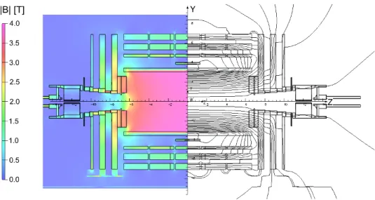
The mapped magnetic flux density on the longitudinal section of the CMS detector is shown in Figure (9). About two-thirds of the magnetic flux returns through the tube yoke, half of which enters the tube directly without passing through the end-cap disks.

Figure 9: Value of magnetic field (left) and field lines (right) predicted on a longitudinal section of the CMS detector.

The Muon Chambers

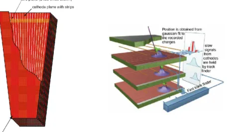
The intersection of the signal from the cathode strips and the signal from the anode wires determines the target positions. The muonton alignment system measures the positions of the DT chambers relative to each other and relative to the entire muonton.

Figure 10: A schematic longitudinal view of one quarter of the CMS detector.

The Forward Detectors

The end cap discs are bent, and the central part of the discs is bent inwards by approx. 15 mm. The CMS alignment system consists of four independent parts: the internal alignment of the tracker, the DT, the CSC systems and the Link system.

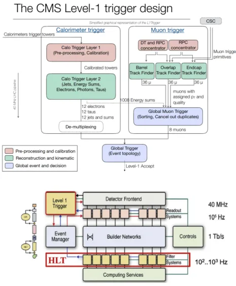
Trigger and DAQ systems

On the other hand, neutrinos do not interact with any of the detectors and are completely invisible. The first one is the reconstruction of the PF elements, which are the tracks, the muon tracks and the calorimeter clusters.

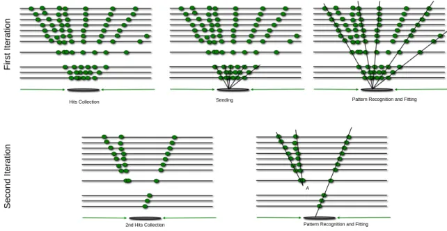
Figure 14: Top: An overview of the L1 triggering system. Bottom: An overview of the CMS triggering system

Track Reconstruction

In the initial iteration, high-pT pixel quadruplets and triplets coming from the beam spot are used as seeds. In the last two iterations, muon tracks were seen from the inside out and from the outside in.

Primary Vertices and Beamspot

The selected traces are then grouped based on their z coordinates at their point where they most closely approach the center of the beam point. The position of the center of the beam point is used, especially in HLT, 1 to estimate the position of the interaction point before the reconstruction of the primary peak, 2 .

Muons

Muon Tracks Reconstruction

Global muons and tracer muons that share the same internal track are combined into a single candidate. Muons reconstructed only as single muon tracks have poorer pulse resolution and a larger mixture of cosmic muons than global and track muons.

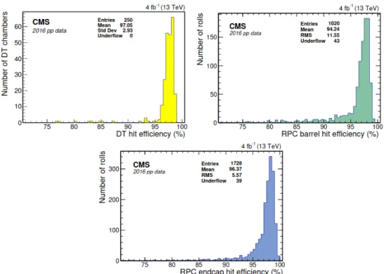
Muon Identification

A soft muon is a tracker muon with a tracker orbit that meets a high purity flag and uses hits from at least six layers of the inner tracker, including at least one pixel hit. These muons are reconstructed both as a tracking muon and a global muon in a similar way to the one followed in the tight muon identification, except for the χ2 cut. The hit reconstruction efficiency for the three types of muon chambers is depicted in Figure (19).

Figure 19: Hit reconstruction efficiency measured with the 2016 data in (upper left) DT, (upperright) RPC barrel, and (lower) RPC endcap chambers.

High Level Triggering Muons

The efficiency as a function of reconstructed muon PT (top left) rises sharply at the threshold. Above 22 GeV, the inefficiency of a few percent is mainly caused by the L1 trigger and the relative isolation criteria. Variations in efficiency as a function of η are caused by geometric features of the detector that affect the L1 trigger efficiency. The isolation requirement accounts for the slight efficiency drop as a function of the number of offline reconstructed vertices.

Figure 21: Trigger reconstruction efficiency [35] as a function of offline reconstructed P T and η measured with 2015 data and simulated events fired Isolated single-muon trigger with HLT P T threshold at 20 GeV

Calorimeter Clustering, Electrons and Photons

The φ window is wider to account for the azimuthal bending of the electron in the magnetic field. To ensure optimal energy containment, all ECAL clusters in the PF block that are linked either to the supercluster or to one of the GSF sport agents are associated with the candidate. This corrected energy is assigned to the photons and the photon direction is assumed to be that of the supercluster.

Figure 23: Electron reconstruction efficiency as a function of η for the 2017 data taking period [33]

Weak Interactions as Gauge Theory

Weak Isospin Doublets and Singlets
Weak Interactions as Yang-Mills Theory
The Cabibbo-Kobayashi-Maskawa Matrix, the W propagator and the
The Z propagator and weak Neutral Currents

Finally, the sum of the polarization states of the virtual photon, which is the propagator for QED, is related to the gµν term. These are hyper-spinors where each of the two components is a Dirac spinor3. Therefore, this finding is the first experimental evidence for the existence of the electroweak theory.

Figure 25: The triple and quartic gauge boson vertices arising from the SU(2) local gauge invariance.

Electroweak Unification

The Higgs Mechanism and the Spontaneous Symmetry Breaking

This Lagrangian is not invariant under the U(1)Y ×SU(2)I local gauge symmetry of the electroweak model. Since the lowest component of the Higgs doublet is neutral and has I(3)W =−12 and therefore the Higgs doublet has, according to (3.36) hypercharge Y=1. To conclude for all the fermions, their mass, the Higgs coupling constant (also called Yukawa coupling) and the vacuum expectation value of the Higgs field υ are combined in the formula.

Figure 31: The Higgs potential for the case of one complex scalar field with µ 2 < 0

Lepton Flavour Universality

R K (µ)

The production process for the B+(B−) meson is independent of its decay mode and the N(B+) is effectively annihilated. 3.66) The first ratio will be calculated from the data and the second ratio will be calculated using Monte Carlo (MC) samples. Finally, this ratio will only be measured on the label side, meaning that only reconstructed muons that have fired at least one trigger will be used to reconstruct the B candidates.

The last four operators are grouped into the third category and are used in electroweak penguin diagrams. For example, b→sl+l− is dominated by C7, C9, and C10, while C8 ranks higher in the strong coupling. Furthermore, only a soft form factor ξP(q2) appears in the amplitude of the heavy-to-light B→K decay due to symmetry relations in the large energy limit of QCD. 3.75) Here, θ denotes the angle between the direction of motion of B and the negatively charged lepton l at the dilepton center of mass frame.

Figure 32: One loop Feynman Diagram for the b→ s transition [28].

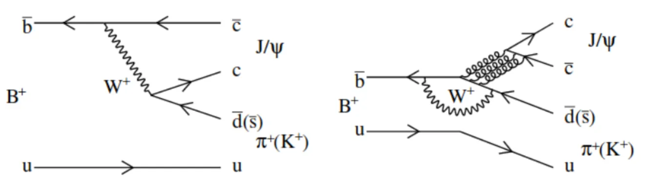
B→ J/ψK

We denote by pB, pK, p− and p+ the 4-momentum of the B-meson, kaon, lepton l and antilepton ¯l, respectively, and MB, MK and ml are the corresponding masses. At high repulsion the energy E of the K-meson is large compared to the typical magnitude of hadronic binding energies ΛQCDE and the squared dilepton invariant mass q2= (p−+p+)2 is low, q2 MB2. The Lagrangian for the transition b →(c¯c)s is given by. 3.78).

Trigger Strategy

This strategy made it possible to capture both the (signal side) muonic and electronic final states necessary for the RK measurements. HLT Mu9 IP6 is the trigger that will be used for measuring RK, as it is the one with the higher statistics and a measurement using the overlap between other triggers is very complex. In both the names of L1 seeds and the HLT pathways, Mu”X” represents the PT threshold of the HLT muon, er”X”p”Y” represents the.

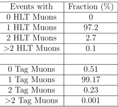
HLT-Reco Muon Matching

As we can see, there is an inefficiency for the multi-HLT muon events, but this is due to spurious HLT muons (tracks created by a single muon) and due to mismeasurements and failed extrapolations from different parts of the detector. As we can see, there is a suppression to positive ∆PT relative values, which means that the PT of the HLT muon is smaller than the corresponding PT of the reconstructed muon. The PT of the reconstructed muons labeled as tag muons is represented in figure (38) (right).

Table 3: Almost 97% of the events passing all triggers have one HLT muon and the rest 3%

Dimuon Mass Region

All candidates in the [2.5,2.9] and [3.2,3.4] GeV regions will be excluded, as radiation tails are expected in these regions. As for the dimuon mass spectrum overlap in the J/ψ and ψ0 resonances, it will be subtracted using scale factor.

B meson reconstruction and preselection cuts

However, not all doublets are used for this process, as we know that the dimuon mass spectrum from the rare mode is extended in the [0,4,8] GeV range. Low PT thresholds for muon and kaon tracks are also used to reduce combinatorics. Some additional preselection cuts are used to reconstruct candidate B, such as the reconstructed requirement PT(B) > 3 GeV or cosα2Dxy > 0, where the angle α2Dxy > 0 is the angle formed by the line segment connecting PV and SV and the reconstructed P vector ~P(B) projected onto a 2D x-y surface as shown in Figure (41).

Figure 41: The reconstructed decay vertex and its properties. The tag muon is labelled with red color.

Therefore, in table (4) the filter factors αf, the fraction of generated B+ candidates with at least one muon exceeding PT >5 GeV and |η| <2.5 over all generated B, because the two decays are listed. The minimum ∆R distribution for the leading and subleading muon and for the kaon is shown in figure (49). In Table (9), the acceptance factor for the subconducting muon and kaon, and the reconstruction efficiency factor × default are listed.

Figure 43: The P T (B + ) and y(B + ) spectra at generation level for the two decays. As we can see the spectra for the two decay modes are identical, which reflects the fact that this spectra are associated with the production mechanism of the B + meson a

BDT training and cut

Therefore, the efficiency factors for massive windows are calculated within the above limits. So we should keep the same slices for resonant and non-resonant modes, but we still need two optimizations, one for the tag and one for the probe side, since the kinematics are different for the two sides. Then, if we integrate an exponential function over the background, we measure the background candidates.

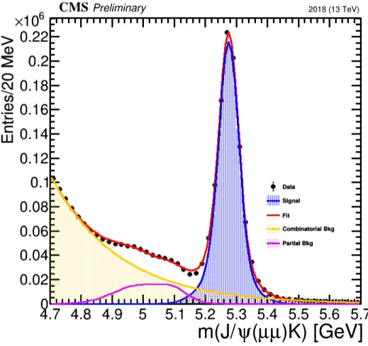
Fitting Processes

The following two parameters (6,7) are the two parameters for the exponential component in the upper sideband. The following six parameters are the amplitude, mean and σ of the two Gaussians describing the partially reconstructed background. The following six parameters are the amplitude, mean and σ of the two Gaussians describing the partially reconstructed background.

Figure 54: Invariant mass distribution of J/ψK ± .

Scale Factor

The first three parameters (0,1,2) are the amplitude, the mean and the σ of the narrow gaussian. The next two parameters (6,7) are the two parameters for the exponential component in the upper sideband. Now, the only unknown value is the number of candidates of the rare mode that have dimuon mass in the J/ψ region, Ndata;rar→J/ψ,.

R K (µ) measurement

According to this MC example, in the low q2 region there are 24394 candidates, while in the J/ψ region there are 7327 candidates.

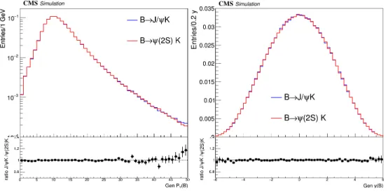
R ψ(2S) (µ) measurement

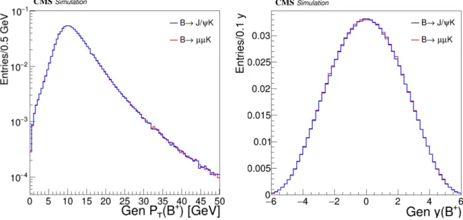
As we can see, the PT spectrum for the J/ψ mode is suppressed compared to the ψ(2S) mode. As we can see, the PT spectrum for the J/ψ mode is again suppressed compared to the ψ(2S) mode. Therefore, after all this, the reconstructed mass spectrum for the ψ(2S) mode is shown in Figure (61).