This thesis was carried out as a result of studies and research carried out for the purpose of exploring the R programming language and in particular its data mining and DBMS connection capabilities. Both case studies sufficiently prove that R is a powerful programming language capable of performing DBMS connectivity and complex data mining tasks.
R
- Summary
- Why use R
- Uses and popular applications
- The R environment
- Commands syntax
- Issuing a command
- R functions
- Vectorization
- R scoping
- Reading commands from external source file
- Importing and exporting data
- Workspace and memory management
- R data types
- Vectors
- Factors
- Matrices
- Arrays
- Lists
- Data frames
- Conclusion
Such a source could, for example, be a network connection over which data can be read using the “read.socket()” function. Finally, reference to an array element can be accomplished using the symbols “[“ and “]” (square brackets), as in most major programming languages.
Data Mining
Introduction
In many ways, data mining is fundamentally the adaptation of machine learning techniques to business applications. Data mining is best described as the union of historical and recent developments in statistics, AI and machine learning.
Data mining phases and techniques
Machine learning attempts to let computer programs learn about the data they study so that programs make different decisions based on the qualities of the data studied, using statistics for basic concepts and adding more advanced AI heuristics and algorithms to achieve its goals. Association mining refers to the process of identifying associations (relationships) between data that occur frequently in the dataset.
Association Rules
- Description
- Rules format
- Interestingness / significance measuring
- The Apriori algorithm
- Association rule mining in R - required packages
- Package installation in R
- Verification of a package installation in R
- Using Apriori in R
- Mining the rules
- Visualizing the results
- Storing the results
The "R CMD INSTALL" command only needs the filename and path of the source code file. The "data" parameter, in short, defines the data set from which the association rules will be mined. The "appearance" parameter instructs the algorithm about the desired appearance of the resulting association rules.
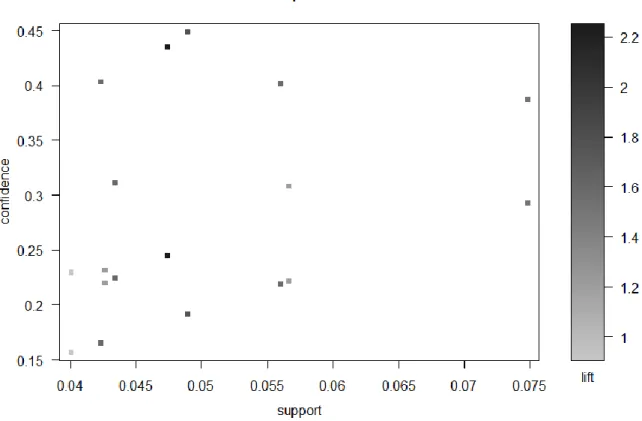
The “default=”rhs” component instructs the algorithm that the RHS of the rule should be the default value (i.e. no restrictions should be applied to it). This example uses a dataset included in the "arules" package, which contains 9835 transactions from a grocery store. So, following on from the previous example, the “plot()” function will be used to create a simple scatterplot of the resulting lines.
In addition to the simple scatter plot, several other visualization charts are available in the “arulesViz” backage. So, to convert a “rules” object to a data frame, the function to use is the “as()” function.
Classification
- Description
- A few words about supervised learning
- Uses / applications
- Classification versus prediction
- The C4.5 algorithm
- Classification in R – required packages
- Using the C4.5 algorithm in R
- Building a decision tree
- Pruning a decision tree
- Visualizing the results
The procedure for loading a package in R and using the “library()” function are described in more detail in chapter 2.3.8 “Verifying a package installation in R”. The rest of the “J48()” function parameters can be specified at will, depending on the desired outcome of the algorithm. For example, the parameter “control” accepts an object “Weka_control”, which can set all the options that Weka provides when building a decision tree.
As can be easily seen from this result, the root node of the tree is “Petal.Width”. The attribute chosen by the algorithm for the root node of the tree is the "Petal.Width" attribute. From the output above, it is easy to see that the “Petal.Width” attribute is the one with the highest information gain and as such is chosen by the J48 algorithm as the root node of the decision tree.
Similarly, two of the observations belonging to the class “virginica” (representing my “c”) were incorrectly classified as belonging to the class “versicolor”. There are two types in which the tree can be visualized, specified by the “type”.
Conclusion
R to DBMS Connectivity
- Introduction
- Required packages
- MySQL
- A short history of MySQL
- Connecting R to MySQL
- Issuing MySQL queries from R
- Fetching information from a MySQL database to R
- PostgreSQL
- A short history of PostgreSQL
- Connecting R to PostgreSQL
- Issuing queries to a PostgreSQL DBMS from R
- Fetching information from a PostgreSQL database to R
- Conclusion
However, most packages depend on a base package, the "DBI" package, which contains an interface definition for communication between R and the DBMS—i.e. Parameters: database connection, table name, and a data frame. (or an object bound to a dataframe) that contains the table rows. Although the fields specified when creating the table were "id" and "name", the table is created with an additional field called "row_names", which contains the names of the table's rows.
Creating a "row_names" field is the default behavior of the "dbWriteTable()" function, and if such a field is not desired, the. The result of the “dbSendQuery()” function must always be stored in an object, to be able to use it to retrieve the result records or close the result set. Most of the functions mentioned above return any fetched data from the DBMS as a data frame.
So, the contents of the remote table "mytable" are now stored in the object "res". Since all the R database query functions are part of the "DBI" package, which both "RMySQL" and "RPostgreSQL" packages depend on, the functions used and the way they are intended to be used are identical, either by querying a MySQL DBMS, or querying a PostgreSQL DBMS.
R installation to the dbTech.net Virtual Machine
- Introduction and purpose
- The DBTechNet Virtual Machine
- Necessary pre-software installation actions
- R setup
- Installation of PostgreSQL
- Installation of required packages
- Conclusion
After successfully importing and uploading the virtual machine, the first thing to do is a plant update, to make sure the package information is up to date, so the latest versions of each package will be downloaded. To initiate a plant update, the "apt-get update" command must be entered in a system terminal. In Debian Linux version 6.0.7, a terminal window can be opened by using the operating system's top menus and going to the.
Once a terminal window is open, root access to the system must be gained, which is accomplished using the “su” command and entering the root password. Once root access to the system has been gained, a CRAN repository must be added to the repository list file before updating the aptitude repositories. The system will now scan all mirrors specified in “/etc/apt/sources.list”.
The total size of the r-base package and its dependencies (that is, the packages that must be installed for "r-base" to work properly) is about 85 megabytes, so it will take some time to download them. After successfully installing R and PostgreSQL, the packages needed to run the case study for this task must be installed.
Case Studies
Mining association rules from supermarket transactions
- Introduction
- Loading the required packages into R
- Pre-processing - reading the transactions into R
- Pre-processing - extracting the transactions information that will be used
- Performing the association rules mining
- Visualizing and evaluating the results
- Storing the results in a database, for permanent storage and further
- Creating a recommender system
- Discussion
To start the procedure, the first thing you need to do is to load all the packages that will be used. So the goal is to create a new relational table that contains the information about the categories of the items purchased in each transaction. First, the tables "articles" and "article_categories" must be created, which will contain the information from the "articles.csv" and "article_categories.csv" files respectively, so that the "items_to_categories" table can be created afterwards.
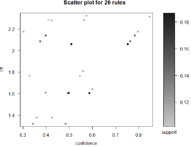
To create this table, all the transactions are required to be scanned, the categories of the items each transaction contains are determined, and a record is it. In this graph, it is clear that the rule located at the top right of the graph is rule number 24 {CONFECTIONERY, FRESH MEAT, PELLERS, FISH} =>. After extracting the association rules, the recommended items for each transaction will be the items contained in the head of the items whose body consists of the items in that transaction.
After recommending the heads of the rules whose bodies consist only of the item purchased by the transaction for which the recommendations are intended, the rules containing more items must be examined. In conclusion, it appears that the relationship between the items of the categories Sweets, BEEF, SAUSAGE, FISH and MILK, CHEESE, EGGS is very important.
Classifying Titanic passengers using a decision tree
- Introduction
- Loading the required packages into R
- Reading the passengers information into R
- Building the decision tree
- Visualizing and evaluating the results
- Discussion
All function parameters are explained in the previous case study, except the 'stringsAsFactors' parameter, which instructs the function to factor all character data read from the dataset. And since all data in this case is categorical, they must be stored in factors - as indicated in the. Once the data from the dataset has been successfully read, the decision tree is ready to be built.
Observing the above output, out of a total of 2201 cases, the tree has correctly classified 1740, corresponding to a percentage of 79.055% of the total cases, while 461 cases have been incorrectly classified, corresponding to a percentage of 20.945% of the total. copies. To create a visual representation of the resulting decision tree, the “plot()” function should be used. Third class passengers seem to be the most doomed: of the 706 people, 528 died.
Observing the outcomes, it can be concluded that most of the crew did not survive (only 212 survivors out of 885 crew members) and about half of the children did not survive either (57 survived out of 109 total children ). ). As for the remaining passengers, a total of 296 women out of 402 survived, but only 146 men.

Epilogue
Rattle GUI is a free and open source software package that provides a graphical user interface (GUI) for performing data mining using R. It is currently used around the world in a variety of situations - currently 15 different government departments in Australia and around the world use world Rattler in their data mining activities, and also as a statistical package. Rattle provides significant data mining functionality by exposing the power of the R Statistical Software through a graphical user interface [24].
Its purpose is to facilitate the use of data mining in R, simplifying many of the actions that must be taken in order for R to perform data mining on a dataset. Although the tool itself may be sufficient for all a user's needs, it also provides a step for more sophisticated processing and modeling in R itself, for sophisticated and unlimited data mining [11]. The interface is tab-oriented; Rattle accepts input from files, and its capabilities include: Calculation of statistical statistics, ability to perform various statistical tests, ability to perform data mining methods such as clustering or classification, ability to visualize the results and the relevant construct models (such as decision trees, for example), the ability to build graphical charts such as histograms or bar charts to effectively represent these results.